View on GitHub
A from scratch build diary. The dead ends, the wrong turns, what went right, and the things I never quite figured out. With no prior metal detector experience, this is where it ended up.
“A low-cost, monostatic time-domain electromagnetic (TEM) spectrometer doing cued interrogation”

1/11/23 Let’s Build a Metal Detector with no Previous Experience
There are heaps of designs and tutorials out there that have given me some great ideas, but as always, I like to start from scratch and design and build a solution to suit me. Although I prefer the digital domain and Python, it’s not going to be fast enough. The maximum sampling I’ve been able to achieve is 50 kHz, or about 20 µs, on an RP2040 running Python. Nowhere near quick enough. I need sub-microsecond samples to make this work, so I’m going to have to do a bit of analogue mixed-signal design.
The basic premise is to capture decaying pulse waveform levels at very specific times: the first one between 1–5 µs after the pulse is removed, and the next between 5–50 µs. Accuracy is absolutely key, so all analogue components will be used up to the sample-and-hold chip (300 ns capture, 100 µs hold). After that, an interrupt will trigger the slower RP2040 ADC reads, which will then store the data sample, synchronised with the GPS position, along with a small telemetry packet to ensure Roverling stays ‘on-mission.’ I’ll probably aim for 10k samples per second.
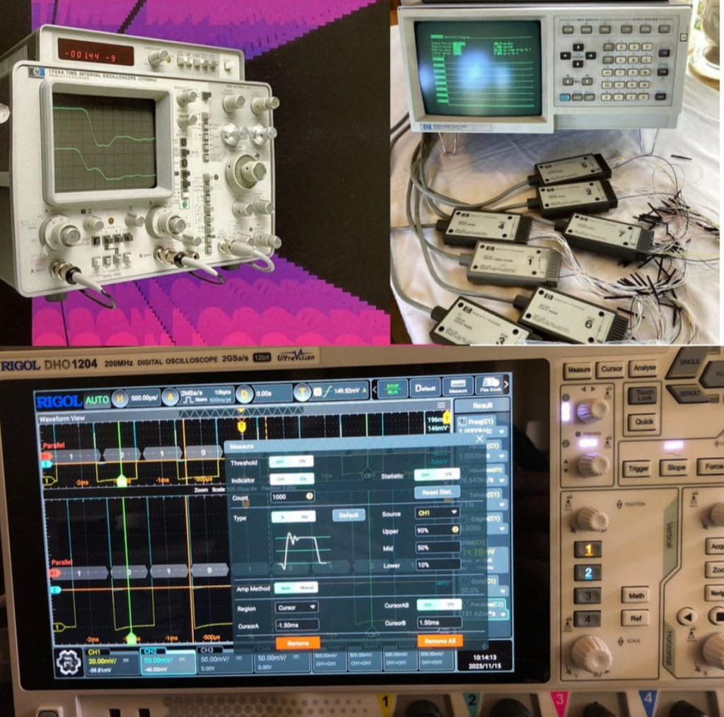
First step, though, is to replace my now-broken cathode ray oscilloscope—it has served me well for many decades. I’ve even got the original brochure. I tried, but it’s just not possible to properly design and tune this system without being able to see what’s happening at a 100 ns resolution. Luckily, my HP1630G logic and state analyser from the same era still works well, although it only samples at 100 MHz.
And it’s time to read some literature, especially since I’ve never even owned a metal detector. The following references were invaluable in this endeavour:
- Inside the Metal Detector by George Overton & Carl Moreland
- Hammerhead Pulse Induction Metal Detector by Carl Moreland
- Making a Fast Pulse Induction Mono Coil by Joseph J. Rogowski
- Coil Basics by Carl Moreland
- Designing Gain and Offset in Thirty Seconds by Bruce Carter (Texas Instruments SLOA097)
- Op Amps For Everyone by Ron Mancini (Texas Instruments SLOD006B)
16/11/23 New Oscilloscope
Christmas has come early—out with the old, in with the new. These old bits of kit have served me well for decades, but it’s time to move on. Thanks to Emona Instruments for the great service and almost instant delivery. I wish I’d had one of these 30 years ago when I was teaching undergrads about metastability—it would have been much easier than trying to adjust the phosphor persistence on a cathode ray oscilloscope.
Next, I’d better download and read the manual.
6/11/23 Design and Construct a Coil
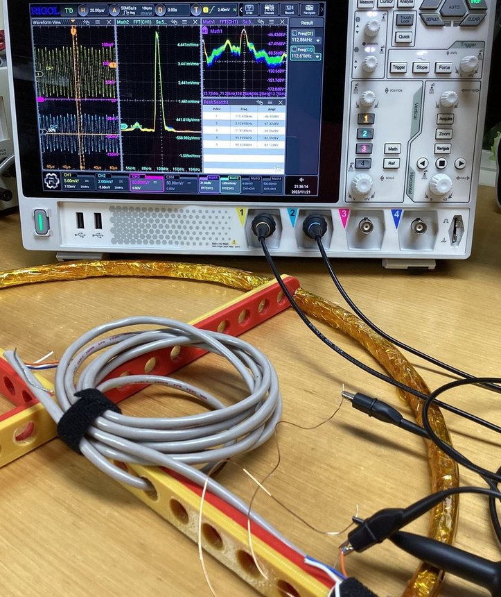
Finally, all my bits are here, so let’s start building a search coil (v2). It’s 400 mm in diameter and constructed from four printed parts that are simply glued together. The inner race has 50 turns of 0.25 mm Teflon-coated silver/copper wire (wire-wrap wire) with an aluminium foil Faraday shield (no loop). This is the receiver and has a DC resistance of 20.1 ohms.
Over the top of the Faraday cage are 20 turns of 0.5 mm enamel-coated magnet wire, with a DC resistance of 2.1 ohms, which forms the pulse transmitter. Then, over the top of that is plenty of Kapton polyimide tape. It looks great on space missions, so why not use it here? (Plus, I no longer need it for holding down ABS prints.)
The next step will be to determine the critical damping requirements for both coils. To that end, I connected the (new) oscilloscope probes to the ends, expecting a 50 Hz signal, but that’s not what I saw. On the scope’s centre window, you can see the spectrum analysis, and that huge spike in the middle? Both coils are picking up something at exactly 118.75 kHz.
You can’t see it in this picture, but about 0.5 m away is my old monitor, which turned out to be fully responsible for this artefact.
Just goes to show that I’ll need an electromagnetically quiet place for calibration and testing.
22/11/23 First Coil – Working?
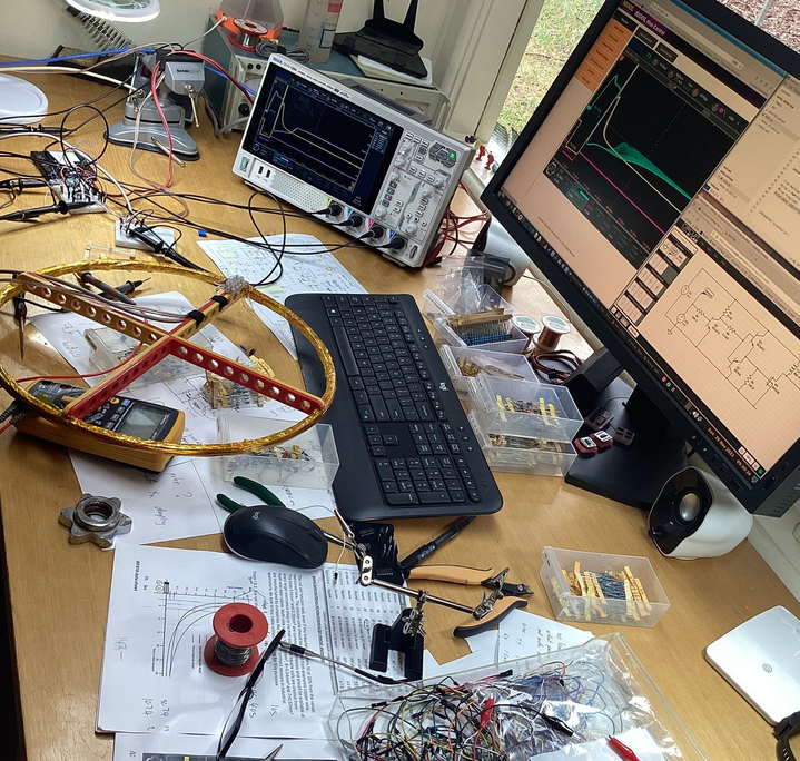
Analogue design is not my strong point, especially when it comes to inductors, but I’ve finally achieved some fantastic results with the coils. Firstly, I needed to create a bipolar totem-pole gate driver for the MOSFET. The parasitic capacitance can’t be overlooked if you want high-speed, non-linear FET switching. I used CircuitLab for the first time to simulate the circuit and was very happy with how quickly I could create the schematic and perform DC and AC analysis. This was critical in my choice of components for the totem-pole, though it wasn’t very useful for coil simulation.
The TX coil pulse is driven by a 100 Hz PWM output from the RP2040, with a duty cycle of 2^16 – 34 at 100Hz, giving a negative pulse of 5 µs. The TX coil needs to be critically damped to prevent unwanted ringing on the RX coil, which I achieved with a 220-ohm resistor. A maximum current of 10 A is realised within the first 1 µs, which suggests this should be the turn-off time. However, I’ve found much better results with a 5 µs pulse at the RX end, with diminishing returns beyond that.
The RX coil is not damped, as I couldn’t see any need for it on my oscilloscope, even though theory might suggest otherwise. The RX output is clipped in both directions using two 1N4148 diodes.
If you look carefully at my computer monitor, you’ll see the aqua (persistent) plot. The top of the envelope indicates no metal, while the bottom of the envelope shows its presence. Without any amplification, the difference is in the order of 500 mV within the 10–50 µs decay time frame.
I couldn’t have hoped for more at this stage.
28/11/23 Wrong Coil Design
Most of the research I’ve done up to this point suggests using a short pulse width, with most sampling occurring in the 5–25 µs decay time frame. However, for my coils, this didn’t seem to provide the large voltage detection swing I was hoping for on the RX coil.
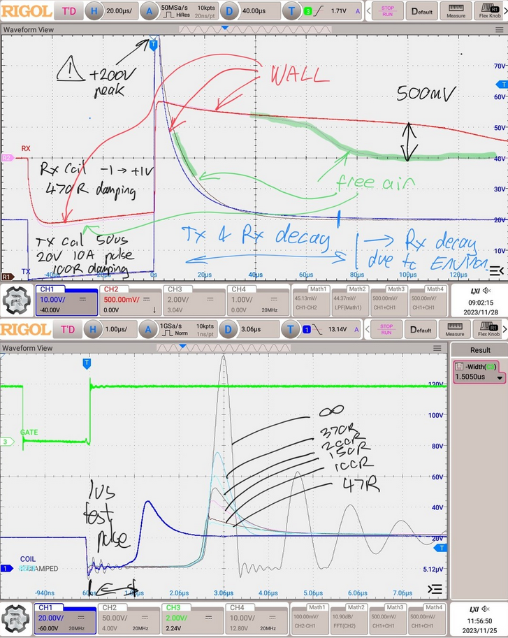
If I drive 10 A through 2 ohms for 50 µs, I get a much better result. The top chart shows the difference in RX coil voltage between free air and a wall with foil sarking. At about 40 µs after the impulse, there’s a massive difference, reaching 500 mV within another 60 µs. Interestingly, there are also detectable changes in the TX coil from 0–80 µs after impulse removal, as well as another change on the RX coil 5 µs into the pulse itself.
There’s a lot of useful information here, but the next step is to test with real dirt and real objects at various depths. I’ll then determine what voltage levels and/or sample time frames to use. Some machine learning could be really useful here. I’d also read that using only an 8-bit ADC wouldn’t provide usable data, but now I’m not so sure. Let’s first see what the RP2040 can achieve before complicating things further.
The bottom chart shows earlier damping tests of the TX coil. This resulted in selecting a 200-ohm damping resistor for the TX coil; HOWEVER, I had to reduce this to 100 ohms to also critically damp the RX coil. I then added specific damping to the RX coil only, which ended up being 470 ohms. Since they effectively form a tuned circuit, I used potentiometers on both until I achieved the desired waveform. Without first tuning (and ensuring your 10x probes are properly compensated), there’s no hope of obtaining the results shown in the top chart.
12/12/23 Getting the Hang of Op-Amps
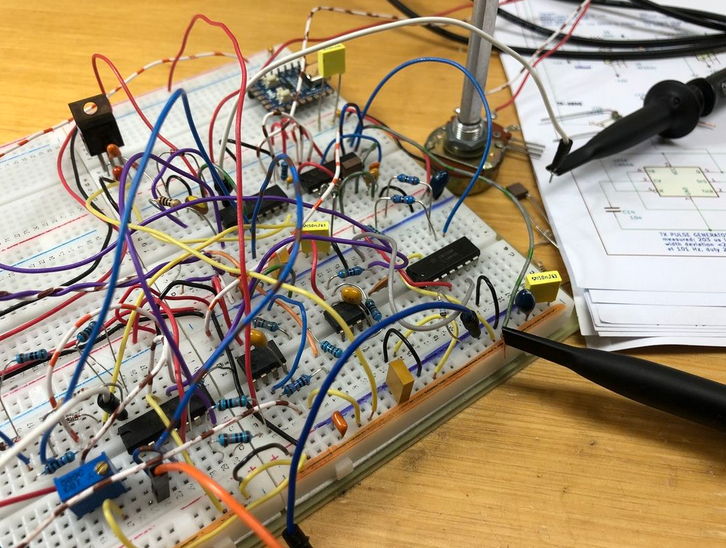
Prototype 1 is complete—but a failure. It can detect a large object at 100 cm, but small close objects go undetected. The biggest mistake? Observing waveforms through ‘rose-coloured glasses’ using all the filtering, smoothing, and analysis capabilities of my new Rigol scope. When switching to high resolution at 2 GS/s and 16 bits, a different story emerges: one filled with noise that completely swamps the signals I’m looking for. Using a long display persistence highlights the problem areas even more clearly.
Now, I’m working on attempt #2 with a much better understanding of op amps. If you’re a rusty engineer like me, you can’t go past Op Amps For Everyone, a Texas Instruments design reference guide (SLOD006B). It’s a tough read but pointed me in the right direction.
The TX coil only becomes fully saturated at about 200–250 µs, so I’m now driving it for exactly 200 µs, resulting in a peak coil current of around 4.5 A. After the RX coil output is clipped to ±1 V, it passes through an NE5534 op amp (primarily an audio op amp) based preamplifier with a gain of 10 and an LPF set at 180 kHz. Next, it passes through another NE5534 with a gain of 13, giving the system an overall transfer function of 30 to 80 mV input maps to -3.3 V to +3.3 V output.
At 60 µs after the end of the TX pulse (but measured on the RX coil), a CD4066-based CMOS switch samples and holds the voltage.
This region (55–65 µs) provides the best signal-to-noise ratio. Sampling earlier than 55 µs results in poorer differentiation, while sampling later than 65 µs falls into the noise floor. Bench testing looks very promising—small objects are now easily detected, noise is largely gone, response time is quick, and I’m getting a clean and held voltage in the range of -3.3 V to +3.3 V. And all of this is working on a solderless breadboard!
The next step is to route this signal into an ADC (after attenuation and level shifting) and bring it back into the digital domain, where I’m most comfortable, for further development.
12/12/23 Learning (but in hindsight looking in the wrong area)
Following on from my previous post, here are the results.
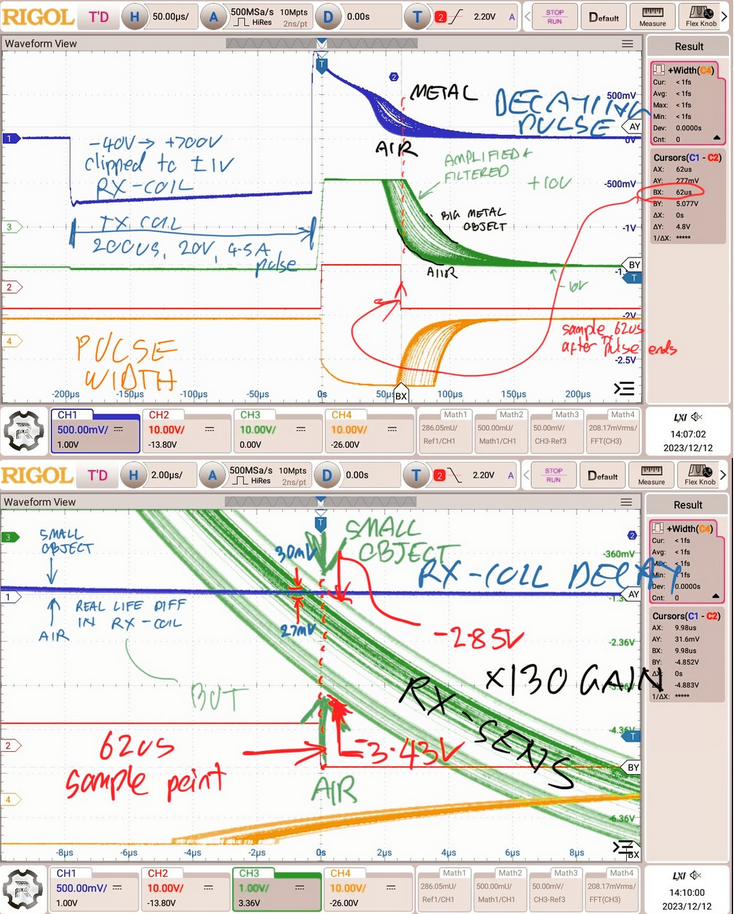
The top chart, at 50 µs/div, shows a very large piece of metal—not a realistic test scenario but still impressive, packing a punch even at 0.5 m. The blue plot shows the received pulse decaying and highlights a sweet spot to measure changes: right at 62 µs after the TX pulse ends.
The second chart zooms in to 2 µs/div. At this level, only the value at 62 µs is relevant. At this point, the RX coil voltage (blue line) for air versus a small metal object is 27 mV and 30 mV, respectively. However, in the midst of the fuzzy noise, it’s nearly imperceptible—just a faint, straight-line difference.
Adding a few op amps to filter and amplify the signal, with a gain of x130, transforms the result into the green line. Now, the readings at 62 µs are 2.85 V for air and 3.43 V for a small metal object—a significant improvement.
4/1/24 Not Happy
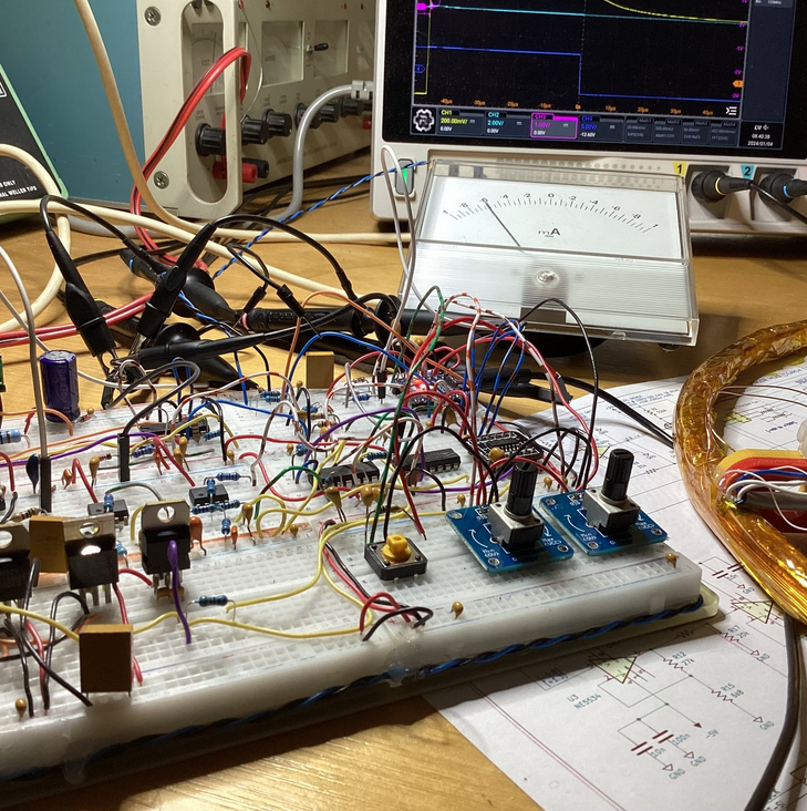
Three prototypes later, and I’m still not entirely satisfied with the design. I can now detect a very small metal object at about 40 cm, but the system’s high gain makes it quite unstable. The RP2040, paired with a bit of Python, helps compensate somewhat, but it’s clear I’ll need something better if I want to fully automate the search process using Roverling Mk II.
Version 3 introduced targeted gain at a specific sample time after the impulse. Right now, the sweet spot seems to be at 47.6 µs, where I’m seeing a voltage change from about 220 mV to 225 mV. The Python code automatically adjusts the baseline, allowing me to amplify just the critical part of the signal. I even display the amplified result on an old-style meter driven by the RP2040 using differential PWM. However, the op-amps I’m using currently have a slew rate of around 13 V/µs, and I’d need something closer to 100 V/µs after amplification to properly resolve the ‘sweet spot.’
Now, Version 4 is on the drawing board. I plan to use higher-performance op-amps (since I now understand them much better) for the input and preamp stages. I’ve also decided to abandon the RP2040’s underwhelming 12-bit ADC. For $30, I can get a 24-bit oversampling ADC with a flat passband digital filter and external sync (critical for my application), with an SPI interface, made by Analog Devices. Honestly, I probably should have taken this route from the start.
11/1/2024 Fly-back Decay Curve
Version 5 is now underway, focusing on a full-scale read of the bottom 5 V of the fly-back decay curve. The coils have been redesigned, thanks to some fantastic online reference materials. Previously, RX coil response sampling couldn’t occur before 45 µs and was more reliable around 65 µs. With this new design—overlaying a circular receive coil under an elliptical transmit coil—mutual coupling has been significantly reduced, allowing sampling to begin at 10 µs. This is a major improvement, particularly for gold detection.
A big thanks to element14 for supplying the precision components. In theory, 32 bits of filtered data over 5 V should provide an LSB resolution in the range of 1.2 nV.
Next problem: these parts no longer come in DIL packages. They’re really small, and I’ll need to solder them by hand… wish me luck!
29/1/2024 Too Small
After numerous attempts to solder 0.2 mm wire onto 0.25 mm pads spaced just 0.5 mm apart, I’ve come to the conclusion that I need SMT-to-DIP adaptors. Luckily, I discovered Proto Advantage. Not only do they have all the adaptors I need for this project, but they’ll also procure and solder those tiny components onto the PCB for me.
Awesome! Now I’m just waiting on delivery from Canada.
30/1/2024 New Coils
Version 2 coils have now been redesigned and are working extremely fast. Even with 2 m of RG62A/U coaxial cable, I can sample down to 7 µs. Discrimination is surprisingly effective, although I can’t test with gold yet since I don’t have any on hand. 🙂 The elliptical coil has proven to be a real game-changer for me.
From my research, most pulse induction detectors only examine the bottom 700 mV of the decay curve. However, in my testing and with my coil, I found the most useful information lies between 500 mV and 5 V. Not only is there significantly more information in this range, but it’s also well above the noise margin, making filtering far easier.
I also examined the response at voltages above 5 V. While I could sample 650 ns sooner in the best-case scenario, this only yielded a 10% improvement—hardly worth the additional effort.
31/1/2024 Finding the Sweet Spot
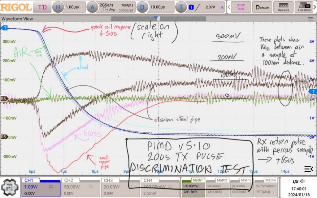
I conducted a controlled test to evaluate the discrimination characteristics of the dual elliptical coil design across various induction pulse periods. The charts display the difference between the baseline and the target object within the 5–20 µs sample period. The vertical resolution is set to 10 mV/div, with a noise component of ±10 mV.
Kicking goals now…
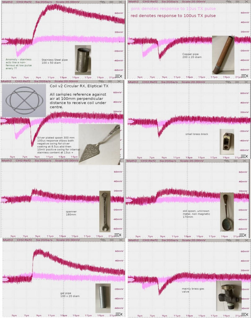
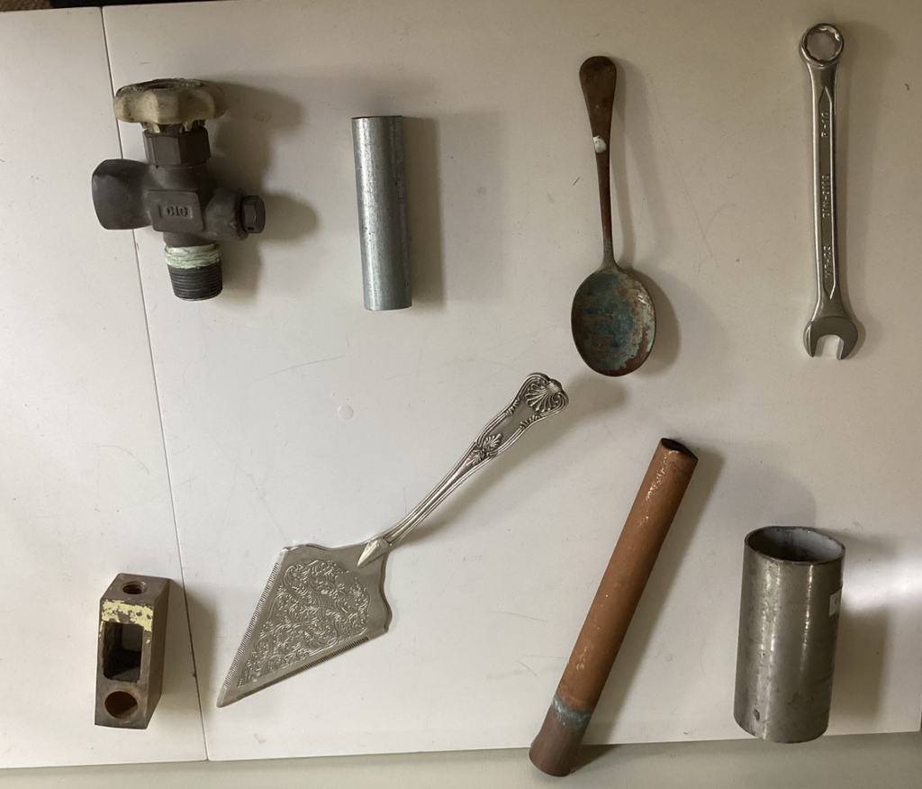
Test objects
2/2/2024 High Voltage
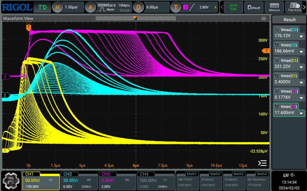
Impulse response versus TX pulse width (h/w/v513) tested with the following increments: first 1–20 µs, then 30, 40, 50, and finally 100 µs.
- Yellow: TX pulse, fly-back reaches 251 V
- Blue: RX pulse, fly-back reaches 176 V
- Pink: Conditioned sample, 5 V max
7/2/2024 Super Fast Sample Time
Automatic sample timing search: h/w v5.14 (RP2040 ADC), s/w v2.08, coil v2.01. The most optimal solution was determined using a natural logarithmic function. With a 5 µs pulse, sampling can begin at 4.5 µs, and with a 50 µs pulse, sampling starts at 7.6 µs, enabling the detection of non-ferrous metals.
The function used:
math.e ** (SampleIndex * 0.3) - 1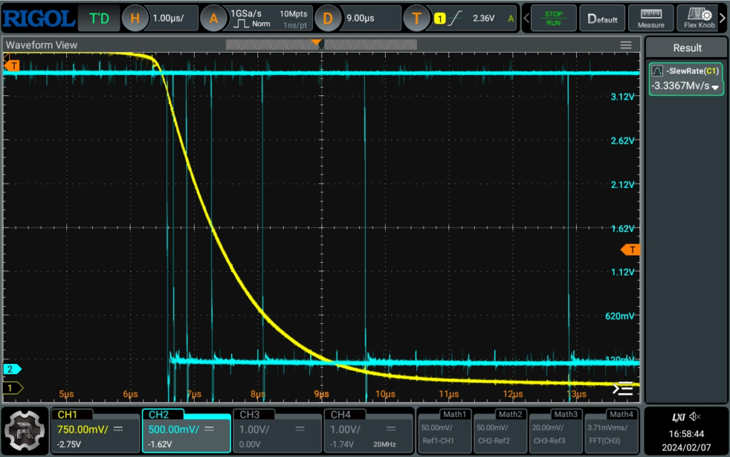
13/2/2024 Integration
The Pulse Induction Metal Detector (PIMD) project now meets Roverling Mk II. Welcome to Stage 2: Integration.
After many months of development, I’ve managed to build a pulse induction metal detector from scratch. While I’m still waiting on better ADCs to arrive before designing a PCB, the PIMD works surprisingly well with the RP2040’s 12-bit ADC. With a transmit pulse ranging from 5–50 µs, I can sample as early as 4.5–7.6 µs, allowing for excellent discrimination between different metals. Taking it a step further, I can also roughly estimate the proportion of ferrous to non-ferrous material.
I’m using an 8×8-LED matrix as an indicator. This effectively serves as a colour-coded bar chart:
- X-axis: Sample time (I take 20 samples, average them, and then apply an LPF at 8 distinct points).
- The first point is determined by searching for the first time the RX return level drops to 95% of the initial detectable voltage.
- The remaining 7 points are spaced using a natural logarithmic function that accurately matches the decay response.
- Y-axis: The difference (in mV) between the current averaged sample and the reference sample.
Precise timing is critical, and I’ve managed to reduce sample timing jitter to under 10 ns. Python on the RP2040 isn’t ideal, as running the PWM frequency at 1 kHz introduces a rounding error (likely), causing 100 ns of jitter. However, switching to 2 kHz resolves this issue. For synchronisation between TX and RX, it’s also essential to use PWM channels from the same slice.
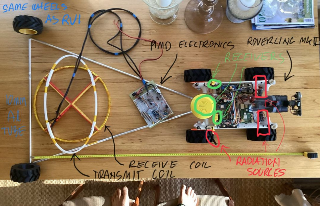
The next step is to integrate the PIMD with Roverling MkII. I plan to use a standard trailer configuration with a tow bar, suspending the sensor coil just above ground level. While I’d prefer carbon fibre or plastic for the frame, I’ll be using 10 mm aluminium rod for now (ensuring there are no loops). Although the PIMD can calibrate around this and maintain a reliable baseline, aluminium in the frame theoretically reduces sensitivity.
Roverling’s onboard electronics present some challenges:
- Noise sources:
- A radio transmitter.
- Two unshielded 11W motors, generating significant interference.
- GPS shielding: The GPS receiver on board is particularly sensitive to pulse noise.
To mitigate this, I plan to position the coils at least 0.5 m from the vehicle. The PIMD electronics, which are also highly sensitive, will be mounted halfway along the trailer for optimal isolation. Additionally, the 40 V vehicle power supply is too noisy, so I’ll be adding yet another Ryobi battery dedicated solely to the PIMD.
Time to fire up FreeCAD and start designing and printing more parts. Let’s get this prototype rolling!
15/2/2024 Massive Power Boost – 6yo Test Driver
Roverling MkII has had its power supply upgraded from 20 V to 40 V to provide the extra torque needed to tow the PIMD sensor trailer up hills. However, with this additional power comes increased speed—so naturally, I handed the controls over to a 6-year-old to test its stability.
Needless to say, I’ll be adding roll bars before any further “junior testing.”
19/2/24 Proto Advantage
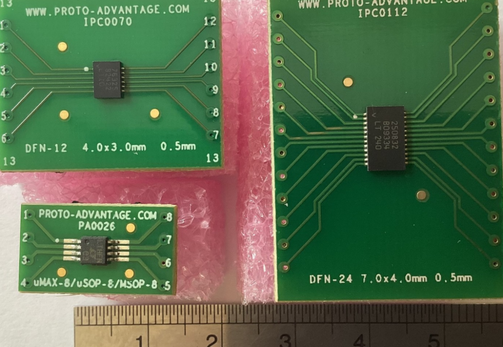
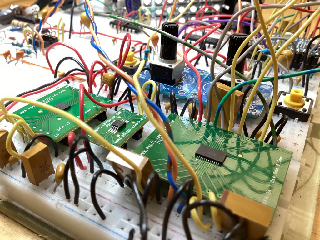
Thanks, Proto Advantage—my parts have finally arrived from the US after three weeks in the post. Looks like my designs are no longer limited to through-hole technology components. Long live SMT!
Not only do they have all the adaptors I need for this project (and likely future ones), but they’ll also procure parts from DigiKey and solder those tiny components onto the PCBs for me.
24/2/2024 Oversample
The new oversampling ADC is now connected and provides two outputs: a 14-bit no-latency value and a 32-bit filtered and decimated value.
The next step was to determine whether the filtered output offers any advantage. The filtering process involves oversampling and decimation by a factor of 256, meaning at 2 kHz sampling, each sample takes roughly 125 ms. Additionally, seven sample periods are required to account for the group delay response to an impulse. This is compared to using eight different sample points at 120 samples per point—significantly more than I had initially planned.
Both methods show a similar response to slow-moving metal objects:
- The first dip is a silver spoon.
- The next bump up is galvanised pipe.
- The final dip is copper pipe.
The vertical scale for this comparison is 11.6 mV/div.
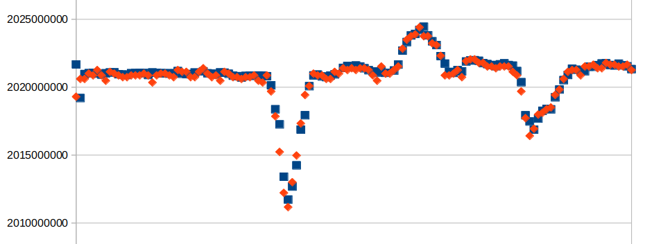
With all other variables held constant:
- Noise in filtered samples (blue) is approximately ±450 µV.
- Noise in raw samples (red) is approximately ±1400 µV.
The left scale represents the adjusted value for 32 bits, where V = x / 2^31 * 5, resulting in 465 µV/div.
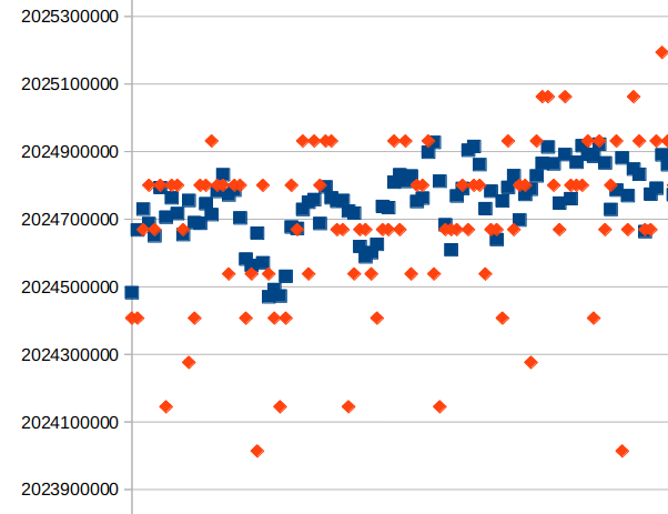
The key decision is whether to pursue multiple sample times or a single sample time with higher resolution. While multiple sample times allow for better discrimination when ferrous and non-ferrous metals are present together, the only significant advantage occurs after the first sample time. Given this, it likely makes more sense to proceed with the single-sample approach for simplicity and efficiency.
26/2/2024 Making Progress
I’ve now coded the system to use the filtered 32-bit data after the initial baselining and sample timing is determined using the raw 14-bit data. The next step was to analyse the characteristics of different pulse widths as an object is passed over a period of 5 seconds. The horizontal axis of the chart represents time, covering about 30 seconds, while the vertical axis shows the integer representation of the ADC filtered value.
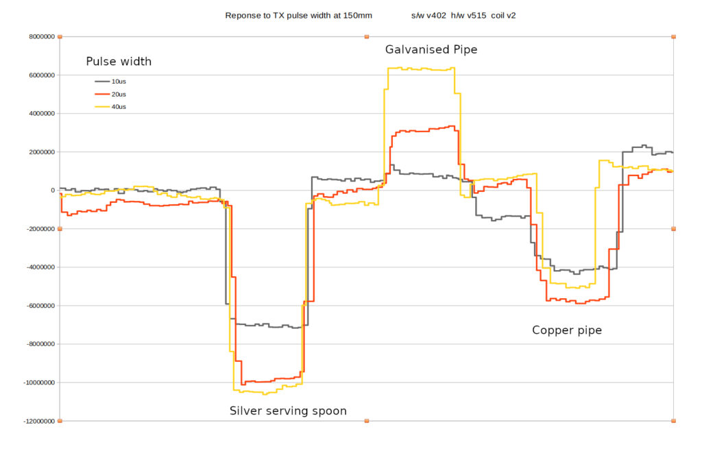
The results so far have been absolutely great! 🙂
- Silver spoon and copper pipe: Both show identical responses for 20 µs and 40 µs pulses.
- Ferrous pipe:
- Almost no response at 10 µs.
- Displays a strange “after-response” when the object is removed.
Increasing the pulse width results in an almost linear increase in sensitivity to ferrous objects but shows only a modest improvement in response to non-ferrous objects.
I’ve traded the ability to collect samples at 8 different points for higher resolution and less noise, but it seems there may be potential for greater discrimination by varying the pulse width. However, there’s one significant challenge:
Heat generation: At higher pulse widths, the system generates more heat. This heat causes slight drifting in the pulse-driving circuitry, which, in turn, leads to substantial drift in the sensitive receive circuitry.
Finding ways to manage the heat and mitigate its effects on circuit stability will be critical moving forward, especially if pulse-width adjustments are to be used for discrimination improvements.
29/2/2024 Printed Circuit Board
It’s time for a PCB before any more fine-tuning to squeeze out those last few percent gains. I suspect the solderless prototype board is now the main contributor to the noise floor.
It’s been 20 years since I last designed a PCB, so there’s a bit of relearning ahead. Back then, I used the very expensive Mentor Graphics software on Apollo Unix Workstations. Now, I’m switching to KiCad—a free, well-supported tool with a large library, running on my free Ubuntu OS on an Intel platform.
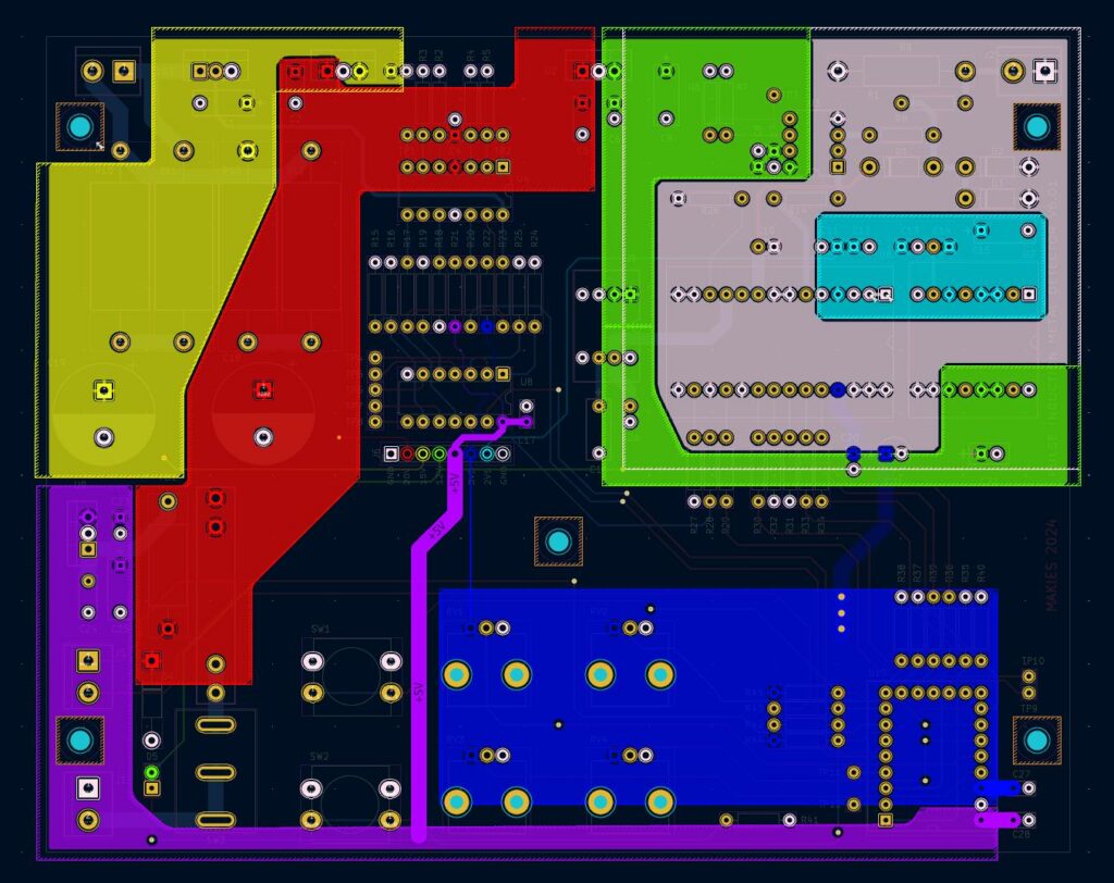
While KiCad doesn’t have an auto-router, I’m not too concerned. I’ve always enjoyed the maze-like challenge of manually routing a tight board. I’m sure there will be plenty of frustrations along the way, but I’m looking forward to diving back into the process.
3/3/2024 Ryobi Battery Problem
Before designing the PCB, I needed to tidy up a few things. First, I shortened the leads to the coils from nearly 2 m (used for testing) to about 50 cm. As expected, this reduced the parasitic capacitance significantly, which was evident because the damping resistor on the transmit coil needed to be increased from 220 Ω to 490 Ω. This, in turn, made the coil even faster—now, with a 20 µs pulse, I can sample as soon as 5.8 µs, making gold detection easier.
Next, I replaced my bench power supply with a Ryobi battery pack, which I use for most of my projects. You’d think a modern battery would be quieter than my ancient power supply, but after a frustrating day of investigation, I discovered that’s not the case.
Every 128 ms, I collect a digitally filtered 32-bit representation of the decaying voltage. Most of the time, the measurements are very stable, with deviations of less than 1 mV. However, every 15 seconds or so, there’s a massive variation lasting about half a second, enough to ruin any accurate detection during that time.
Here’s an excerpt of the data:
  10866ms  0x6a797184   4.1591558456V   diff:  -0.531mV
  10988ms  0x6a7ae6b2   4.1593780518V   diff:  -0.309mV
  11131ms  0x6a79da94   4.1592183113V   diff:  -0.469mV
  11254ms  0x6a77b9d9   4.1588935852V   diff:  -0.794mV
  11377ms  0x6a773a09   4.1588172913V   diff:  -0.870mV
  11500ms  0x6a781620   4.1589488983V   diff:  -0.739mV
  11642ms  0x6a680a63   4.1565003395V   diff:  -3.187mV
  11765ms  0x69c88efc   4.1321654320V   diff:  -27.522mV
  11888ms  0x688ad5af   4.0836844444V   diff:  -76.003mV
  12011ms  0x687c80b7   4.0814976692V   diff:  -78.190mV
  12154ms  0x69b79a6b   4.1295781136V   diff:  -30.109mV
  12276ms  0x6a64f890   4.1560320854V   diff:  -3.655mV
  12399ms  0x6a799e2b   4.1591825485V   diff:  -0.505mV
  12542ms  0x6a797779   4.1591591835V   diff:  -0.528mV
  12665ms  0x6a7891de   4.1590223312V   diff:  -0.665mV
In the measurements above, you can see the stability in the data, followed by a sudden, massive variation.
I connected the oscilloscope to the Ryobi battery pack, and even with no load, the battery exhibits a strange behaviour every 15 seconds. It appears to be performing some kind of internal check.
The yellow line marks the end of the excitation pulse, the green line represents the last 5 V of the received decay, and the rising blue edge shows the exact sample point. With persistence turned up, you can clearly see shadows in the transmit and receive pulses dipping briefly—enough to interfere with accurate detection.
Zooming in on the spikes reveals that each event lasts around 1 ms, with a voltage drop of nearly half the battery’s total voltage.
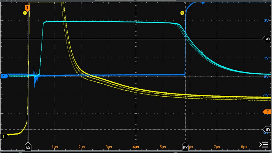
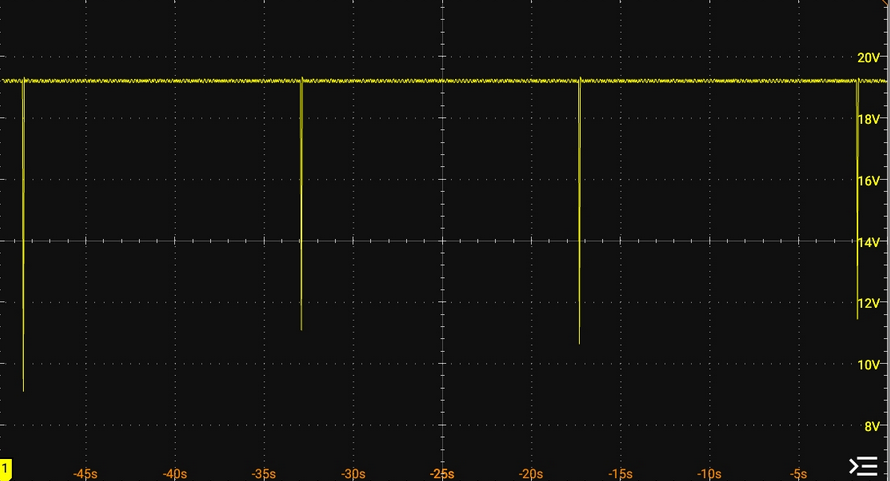
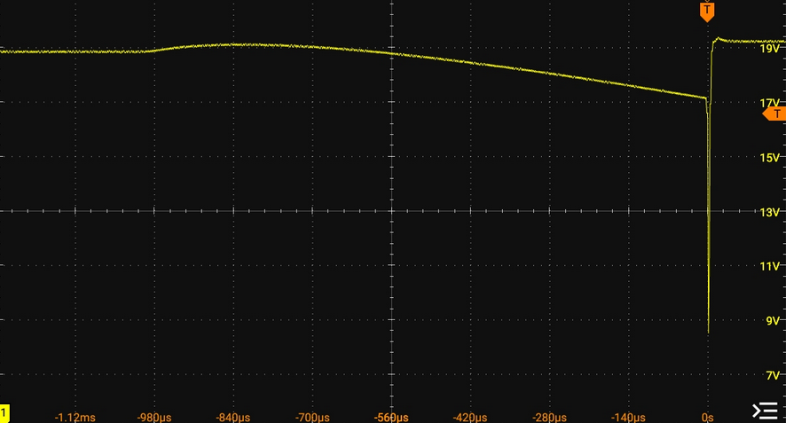
The Ryobi battery pack is clearly unsuitable for sensitive applications like this. I’ll need to find a quieter, more stable power source for this project. No more Ryobi battery packs for precision work!
9/3/2024 Drift
Next problem to solve – drifting component parameters, especially when going to full power on the drive circuitry. This phenomenon doesn’t work well with the static baselining I have been doing up to now, but it has its place for pinpointing edges so I’ll keep it in the system.
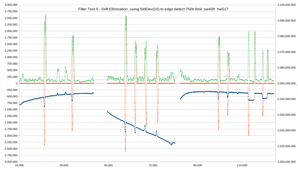
What I really thought I needed was a high pass filter. I found a much better solution using statistics, in particular the standard deviation function. In the below chart, the blue line is the filtered/decimated ADC 32 bit data, decimal scale on the right axis. The green is the standard deviation, and the red is the standard deviation multiplied by the sign of the difference of the sample at the beginning and end of the sample. Bottom scale is time in ms.
From left to right, first blue run with 20us pulse, passing samples at 150mm Ag, Fe, Fe, Ag. Next run turned up pulse width to 50us which heats up the power resistors somewhat. I didn’t wait for it to stabilise so drift down is evident. Samples Ag, Ag, Fe, Fe. You’ll notice a much bigger response to ferrous metals. Last run turned the pulse (effective power) down to 5us. Samples Ag and Ag followed by a hold over samples Ag & Ag.
In the chart below:
- Blue line: Filtered and decimated 32-bit ADC data (right decimal scale).
- Green line: Standard deviation of the data.
- Red line: Standard deviation multiplied by the sign of the difference between the sample values at the start and end of the sample window.
- Bottom scale: Time in milliseconds.
- First Run:
- Pulse width: 20 µs.
- Passed samples: Ag (silver), Fe (iron), Fe, Ag.
- Stable operation, minimal drift.
- Second Run:
- Pulse width: 50 µs (increased power).
- The power resistors heated up, causing noticeable drift (downward trend in the blue line).
- Passed samples: Ag, Ag, Fe, Fe.
- The response to ferrous metals (Fe) is much larger with the increased pulse width.
- Third Run:
- Pulse width: 5 µs (reduced power).
- Passed samples: Ag, Ag, and then, Ag, Ag but slowly.
Using standard deviation and its signed adjustment provides a dynamic way to account for drift, without relying solely on static baselining.
Increasing the pulse width significantly improves ferrous metal detection, but it also introduces drift due to component heating. Conversely, shorter pulses reduce power consumption and drift but provide smaller signals.
14/3/2024 Power System Noise
Following on from the Standard Deviation edge detector, I’ve implemented a simple state machine to better detect changes and their direction. Now that this has been refined, it works very well up to about 20 cm, after which the noise becomes significant. It’s time to work on reducing noise, even though I’m still using a solderless breadboard.
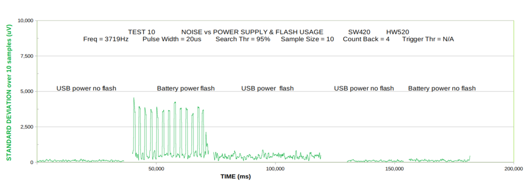
The plan was to untether the USB connection used for code development, but that turned out to be harder than expected. Initially, I used the RP2040’s onboard flash memory to store data while disconnected, but this caused at least a 10-fold increase in the noise floor, even with an additional half dozen capacitors added. Once I identified the issue, I configured a single UART TX pin to output the data instead, eliminating the need for USB connectivity or onboard flash storage.
What surprised me most is that noise is about 50% lower when the RP2040 is powered via USB—either from a PC or a plug pack—compared to using the onboard 7805 regulator with the 20 V supply. Nothing I’ve tried has resolved this, and I suspect a proper PCB may help reduce the noise further.
Another major improvement came from changing the pulse and sampling frequency. I was initially using 4 kHz, but since it isn’t a prime number, there seemed to be a beat frequency in the noise. Changing to 3719 Hz reduced the noise by half.
Current baseline noise standard deviation over 10 samples in free air:
- 200 uV USB powered, no flash
- 250 uV Battery powered, no flash
- 900 uV USB powered, using flash
- 4000 uV Battery powered, using flash
16/3/2024 Critical Component
I accidentally blew up a critical component due to my dodgy solderless breadboard and loose wires. While I wait at least three weeks for the SMT replacements to arrive from Canada, I’ve decided to bite the bullet, relearn PCB design using KiCad, and finally get a proper PCB designed and manufactured.
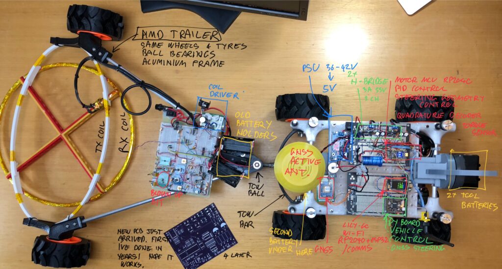
30/5/2024 Creating Roverling Vehicle Control System
While waiting for replacement components, I began work on RV3, an updated version of Roverling based on the previous MkII, but specifically designed to operate autonomously with the metal detector.
It’s almost complete, but outdoor development has stalled due to rain. One of the final tasks is achieving accurate GPS steering. At the moment, I can achieve about 0.5 m accuracy, but for this project, I’ll need a GNSS RTK-capable module. I’m currently searching for a good but affordable option.
Fortunately, there are a couple of nearby government Continuously Operating Reference Stations, and their free NTRIP correction streams should allow me to achieve 2–3 cm accuracy.
8/7/2024 Roverling in Control
It’s taken some time, but the Roverling control system is now working well.
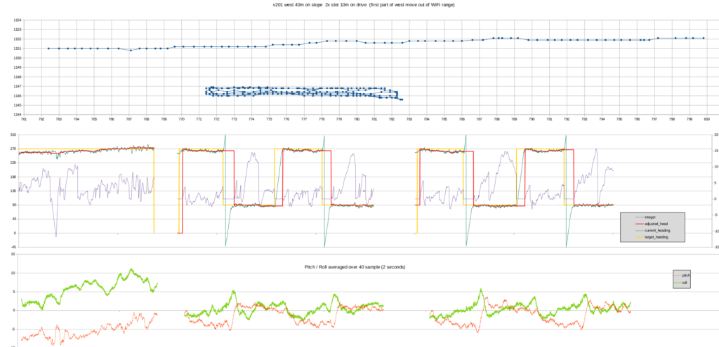
The first level of control uses a magnetometer, calibrated offline using all three axes for sphere re-mapping, and then calibrated again on the Roverling itself using only the X and Y axes with a figure-of-eight manoeuvre. However, the magnetometer is only accurate when horizontal, which is problematic when Roverling is navigating up, down, or across hills. To address this, tilt compensation is applied based on pitch and roll, which are derived from a three-axis accelerometer. Unfortunately, the accelerometer can only determine pitch and roll while stationary, which isn’t helpful when moving.
The next level of control comes from the GPS. While helpful, there are still limitations until I can integrate an RTK module. For now:
- The best update interval is once per second.
- Precision is around 18 cm.
- Accuracy, after locking onto approximately 20 satellites and allowing 15 minutes to stabilise the fix, is about 50 cm.
While there’s room for improvement, the system is good enough for now.
The chart below shows GPS position during fully autonomous control:
- First test: A 40 m run on a varying 10-degree slope. Roverling stays within a 1 m corridor.
- Second test: A series of ‘slots’ on flatter ground, 10 m long, with tight turning circles at each end. Again, Roverling maintains a 1 m corridor.
It’s a promising start!
12/7/2024 PCB Arrives
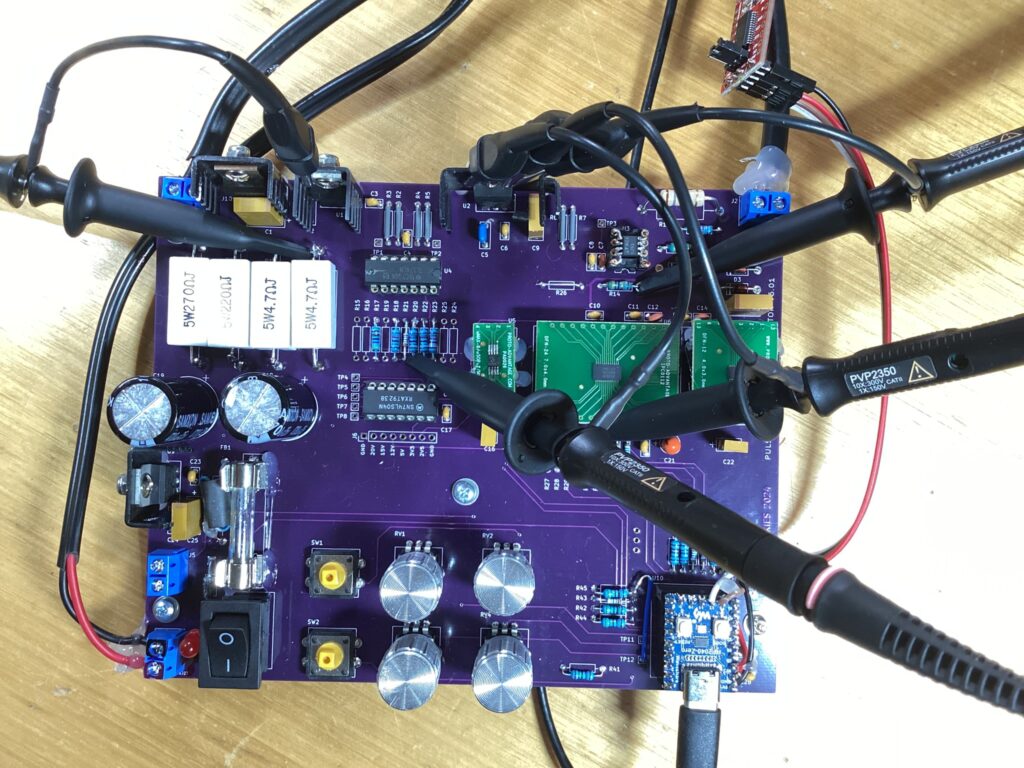
The first PCB I’ve designed in many years has arrived and is working with only a few minor issues. I’m now in the process of testing and calibrating it.
So far, it looks like I’ve managed to achieve a minimum sampling delay of around 4 µs and approximately 10 µV of precision on my timed 32-bit ADC sampling.
A great step forward!
1/8/2024 First Integration Test
The first integration test is complete! The power systems are working well, and RS232 communications between the PI trailer and Roverling are solid. I’m getting 30 updates per second from the PI’s 32-bit ADC via LoRa, streaming back to my desktop computer.
However, there’s an issue: it seems the coils are too loose, and the wires are shifting relative to each other during the shaking and bumping. To address this, I’ll coat the wiring in epoxy to stabilise it and also work on making the trailer lighter.
A few more tweaks, and it should be ready for further testing!
23/12/2024 New Coil Design – Version 3
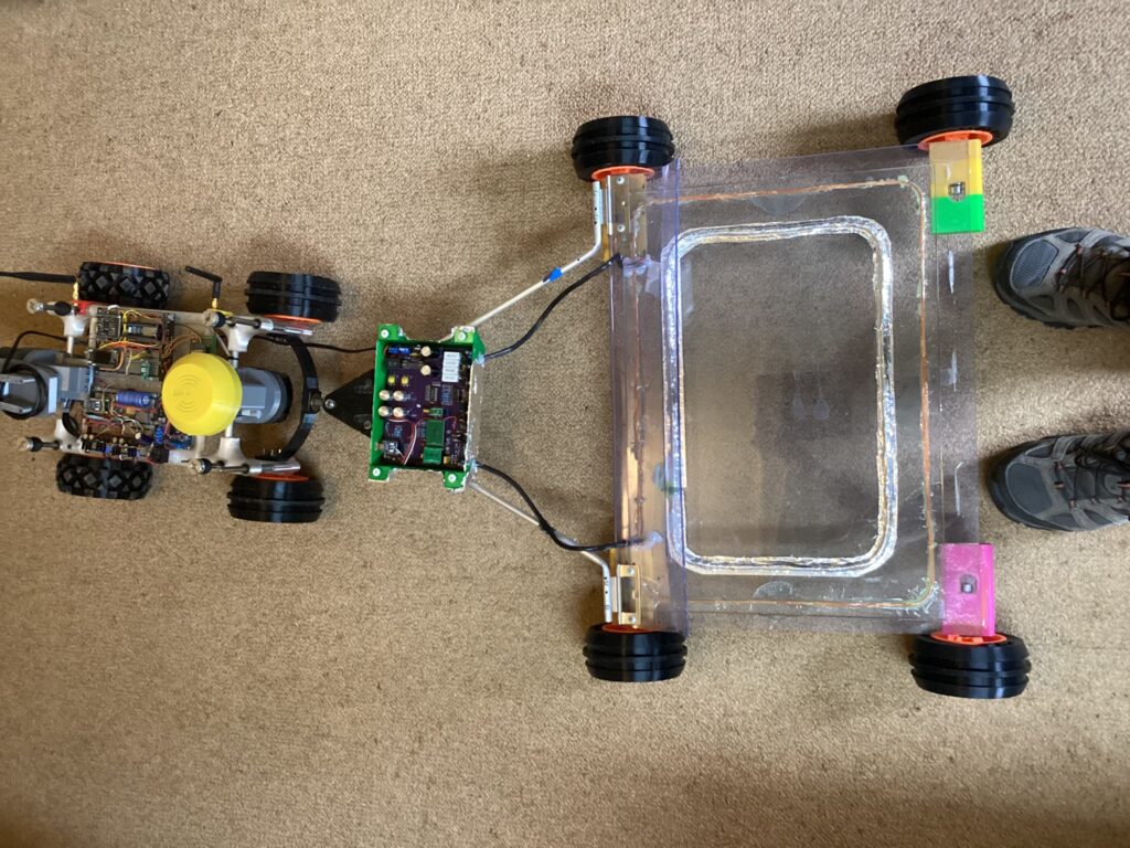
I’ve gone back to basics with a version 3 coil, focusing on making it stable. This design consists of two rectangular coils epoxied onto a 6.25 mm glass substrate, protected underneath by a polycarbonate sheet.
- Transmit Coil:
- Dimensions: 520 x 360 mm
- 10 turns of 0.5 mm (24 AWG) enamelled magnet wire
- Length: 17.6 m
- Resistance: 1.7 Ω
- Receive Coil:
- Dimensions: 430 x 265 mm
- 50 turns of 0.25 mm (30 AWG) Teflon-insulated, silver-plated copper wire-wrap wire
- Length: 30.8 m
- Resistance: 22.9 Ω
Many designs I’ve seen include a series resistor in the drive circuit for the TX coil. I experimented with this and found that reducing the resistor from 9.4 Ω to zero only slowed the response by 0.6 µs but significantly increased depth penetration.
Although this version performs well on the bench, it’s very heavy, and the front-wheel-drive Roverling struggles to maintain traction. I’ll need to revisit the design to reduce the weight while maintaining stability.
2/1/2025 New Coil Design – Version 4
I’m exploring alternative materials and techniques to develop a better solution for keeping the coils rigid while reducing weight.
The Version 3 coil, while stable and functional, proved to be too heavy for the front-wheel-drive Roverling, causing traction issues.
The goal is to maintain stability and durability without compromising the performance gains achieved in the previous version. Time to get prototyping!
16/2/2025 Field Tests
Coils v4 is now complete. I used a piece of 12mm thick perspex and had slots routed to house the coils. The receive coil is shielded by copper tape, and then both coils are embedded in perspex. For the initial field testing I’ll use this ‘pusher’ and a laptop to monitor using this newly created GUI.
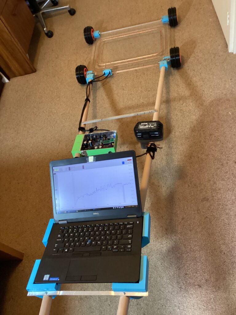
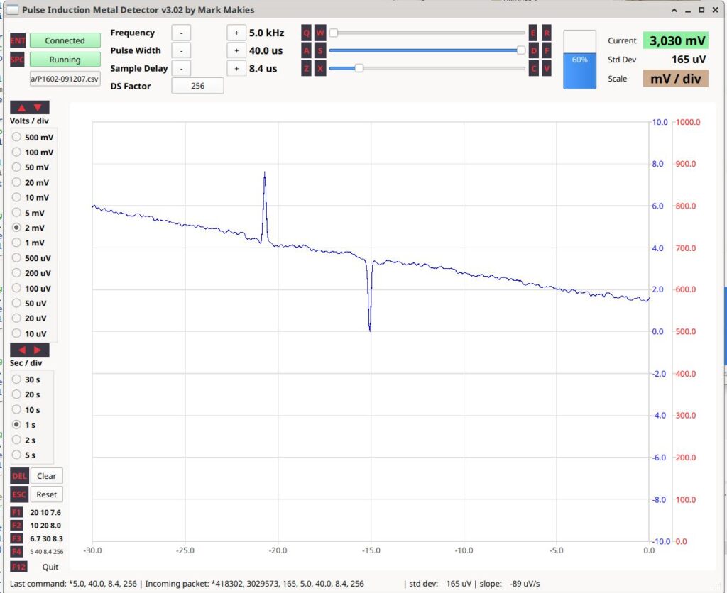
I have now developed a Python-based GUI to interface with the RP2040 acquisition MCU. The timing between the removal of the transmit pulse and the subsequent acquisition of the receive pulse is accurate to within 15 ns. Once the coils and circuitry have warmed up, the standard deviation of the received signal is typically better than 100 µV.
The slope seen in the data below is due to the system still warming up. Nonetheless, it’s clear that ferrous metals (steel spanner) are detected as positive spikes, while non-ferrous metals (piece of copper pipe) produce negative spikes. The polarity difference happens because ferrous metals store magnetic energy, reinforcing the decay field (positive spike), while non-ferrous metals induce opposing eddy currents, weakening the field (negative spike).
Through testing, I’ve found that the optimal setup is a 40 µs transmit pulse, generating a peak current of 7 A. Sampling at 8.4 µs provides the best results, as this is when the 100V+ signal has been critically damped to around 3V. The system runs at a 5 kHz pulse rate, with a decimation filter of 256, providing 20 samples per second.
I’ve already detected a few large underground spikes but haven’t dug them up yet to see what they are.
22/6/2026 — Back from the Shelf
It’s been over a year since my last entry. I kind of lost interest and got busy on other projects.
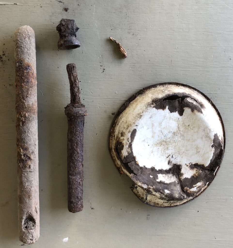
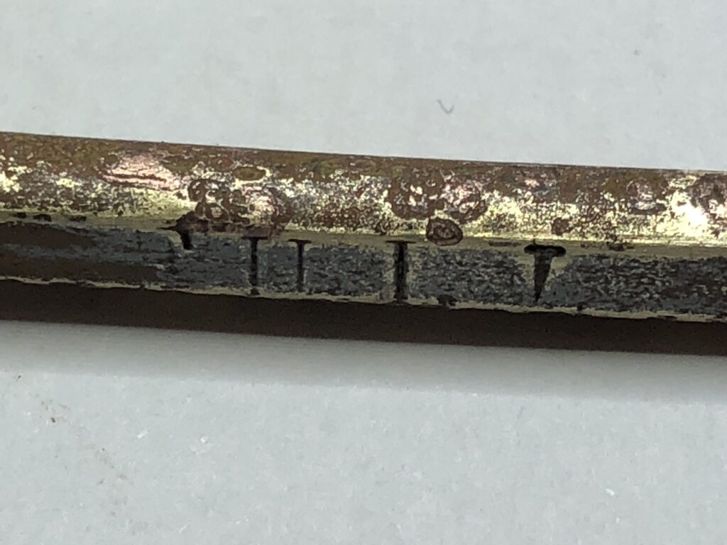
Where I left off it actually worked in the field. I found a 90-year-old brass dipstick about 30cm down, an old buried enamelled steel plate and some sash window weights, pushing the coil on wheels around and watching the laptop. No real ground discrimination, just doing it manually from the GUI.

Then a couple of things happened that completely changed the trajectory.
For a very short period I got access to Fable 5, Anthropic’s newest model. I wanted to give it a real test, so I looked through my project directory for something meaty and maybe unfinished. I found PIMD and thought that will do. I fed in the Python source code, all my notes, this diary, schematics, screenshots, oscilloscope plots, etc. I then asked Fable to do a deep review against commercially available equipment, specifically pointing out good and bad points. Was I even in the ballpark?
It pointed out some flaws, but also uncovered things I wanted to do but didn’t — mainly because of the programming effort required. I knew I would be fighting Python at this level, and it would take me forever. But the other thing I have wanted to do for a while was to learn how to use Claude Code.
So inside a week all the bugs and mistakes with my firmware and GUI were sorted out, and new functionality added, which I could never have done myself in a reasonable time. Two new PC apps were created: pimd_delaycal.py, which automatically determines exact timings for acquisitions, and pimd_classviz.py, a tool to visualise the data.
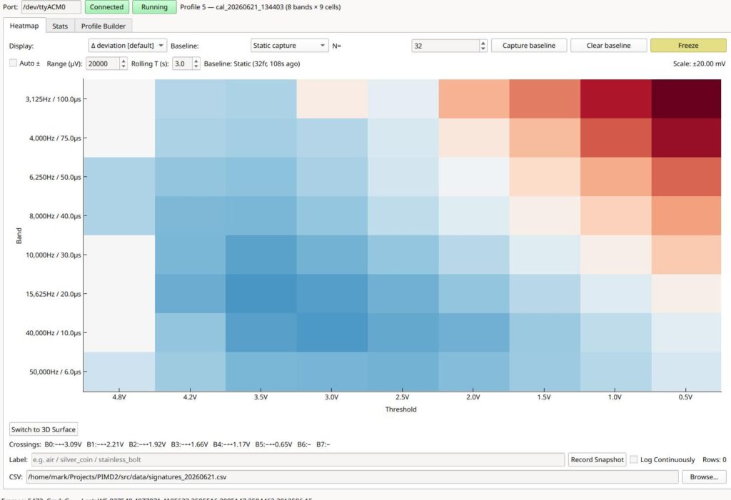
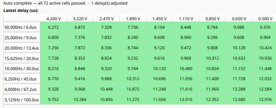
Below pimd_classviz.py heat map chart showing both a ferrous (red in upper right) and non-ferrous (blue lower left) targets under the coil simultaneously. The X axis shows target voltage rather than sample delays as they are different per power band. They vary from 6.272 us to 12.976 us.
I’ve decided to publish everything to date on GitHub: the firmware, the three PC tools, the KiCad project, a full engineering reference and the per-tool docs. It’s a work in progress, but someone may find it useful.
There’s some refinement to come, possibly trimming the cell count for a faster response, but only once I’m certain I’m not throwing away hidden information in those extra cells, and a front-end revision to retire a 1990s MOSFET I’ve been running rather harder than its data sheet would like. And one day design a proper PCB.
So much has changed in the update – best to consult Change Log in GitHub to get up to speed.
3/7/2026 — Time to Tune
I started tuning using Delay Calibration utility and settled on geometric spacing of pulse widths and voltage dependent target sample points. This change from my linear arrangement should allow me to capture more ‘valuable’ data.
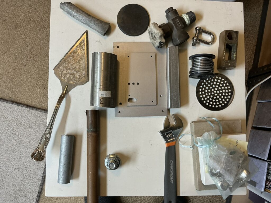
And I started profiling the targets and 5, 10 and 15 cm range. A mixture of what I have at hand, some materials not entirely known.
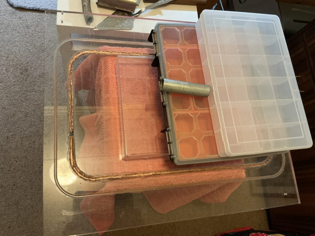
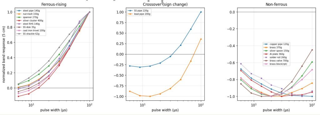
The big result today is that a target’s signature shape stays same, within a few percent, as it moves away from the coil, only the strength changes. Even better, the same object measured in different sessions, and even under a different calibration, gives the same shape to within a few percent. The signatures sort themselves into three natural families: ferrous (signal grows steadily with pulse width), non-ferrous (opposite sign, peaking at shorter pulses), and a surprisingly common third class of “crossover” targets — cast iron, stainless pipe, real jewellery, that read non-ferrous at short pulses and ferrous at long ones.
15/7/2026 — Time to Train
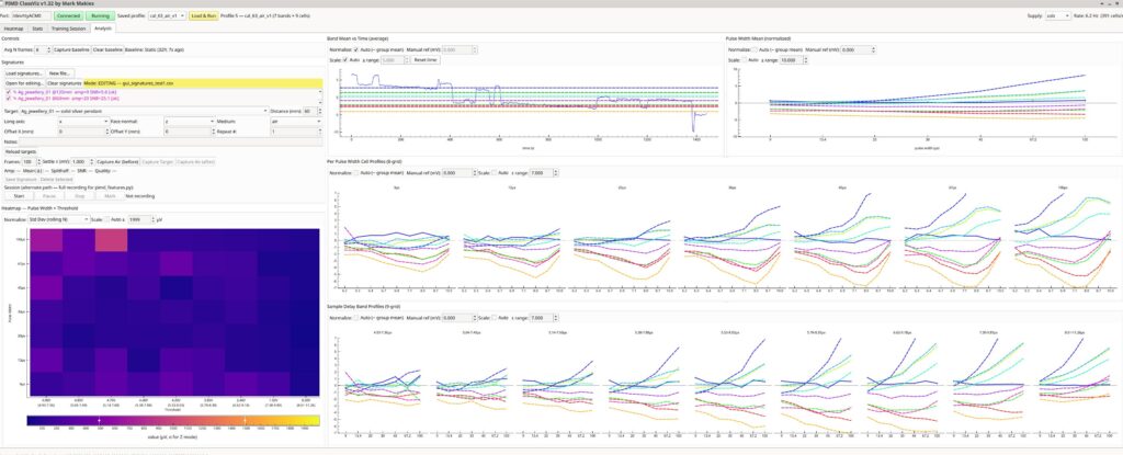
I’ve gone back a few steps and fixed multiple small bugs in MCU and desktop code. These were found whilst trying to capture reliable training data – glitches here and there and boundary/edge issues were corrupting the data. I’ve now created a library of target parameters which includes size, shape, material, etc. I’m developing the training corpus using the analysis screen, where I can state distance, orientation, medium, etc. I have 100s of samples to take, and then it is all about analysis of results. Early results look promising. Below is the first few targets mapped a few different ways. It is clear that the different targets have very different responses.
I’ve also thrown out the geometric progression and instead used the charts to determine optimal spacing points. Exact timing is in the repo, but for example at a 20us pulse excitation width, we sample at 5.816,5.936, 6.048, 6.312, 6.456, 6.72, 7.576, 8.256, 9.576, which gives target voltages of 4.9, 4.8, 4.7, 4.4, 4.2, 3.8, 2.4, 1.5, 0.5.
Now these may look like pretty exact timings, and they are. We have 8ns resolution (from the MCU 125MHz clock), and every 8ns steps the response by a whopping 10mV. Also note that the rig is still warming up, hence the gradual rise.
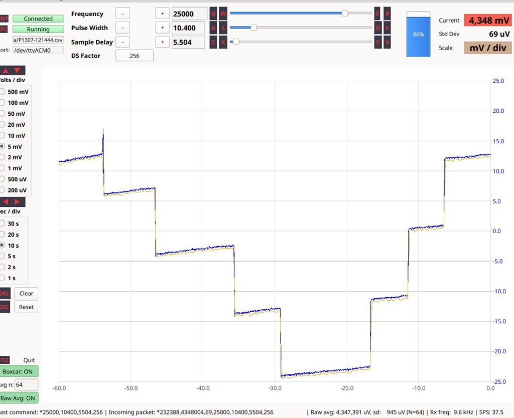
Note there is a big gap between 4.4 and 4.7V. This is due to the 1N4732, a 4.7 V zener diode that limits front end voltage to the op-amp. This keep out range sits were the zener crosses over between true-zener and avalanche-conduction. It’s a soft knee and it is particularly noisy – in fact about 10x the surrounding cells, so we just keep out of that range for now.
24/7/2026 — Family Plane
Yesterday I finally went through the long task of profiling 22 objects at at least three distances each, out to 360mm. I shoved the numbers into Claude and we found a new metric:
Take each signature, normalise it, and plot just two numbers: the average response at short pulses (9–13 µs) against the average at long pulses (67–100 µs). Every target lands in a quadrant. Non-ferrous bottom-left (negative at both ends), ferrous top-right (positive at both), and the crossover targets — cast iron, stainless, galvanised tube — top-left: negative early, positive late.
Sorting targets by family this way is about 98% reliable if the signal is well clear of the noise floor. And the shapes hold: the same object gives the same signature, typically within a couple of percent, as it moves away from the coil — only the strength changes.
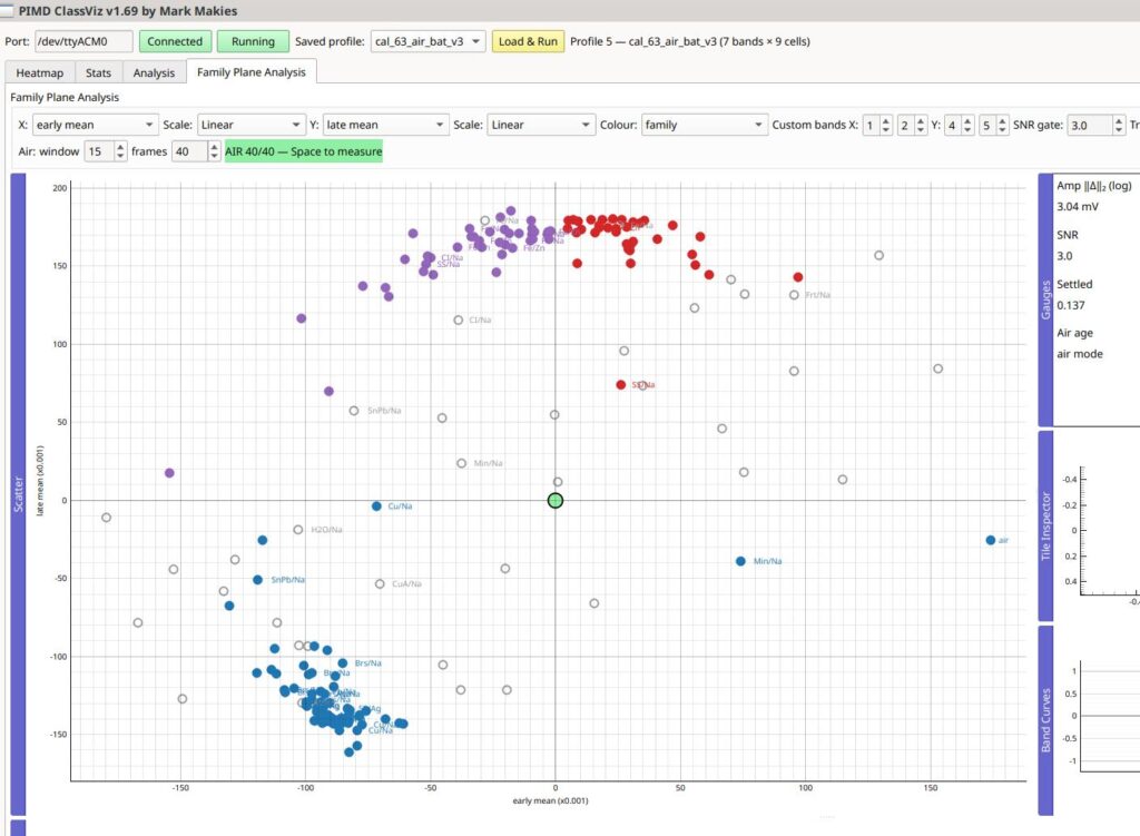
And then we found another very valuable measure in the middle band: the pulse width at which the signature crosses zero. The charts tell the whole story.
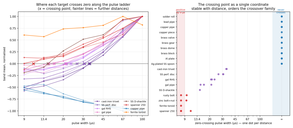
Now this is getting interesting, a PI metal detector with good discrimination (in air anyway)…
1/8/2026 – Orientation, not Material
Since the last entry the corpus went from 66 captures over 22 objects to 188 captures over 25, across eight sessions and three days. The important difference isn’t the size, it’s that this one deliberately spans orientation, every target captured lying flat and stood on edge.
In my last post I was pretty pleased with 98% on ferrous / non-ferrous / crossover. But that number was bullshit, it was actually measuring geometry / orientation. I added a tilt input and captured the trivet and a stainless disc at 0, 30, 60 and 90°. Every oblique capture turns out to be a straight positive mix of the flat and edge-on signatures. The mixing weights land on the textbook dipole prediction, cos²θ and sin²θ, to within about 0.015.
However, the other axis, the late-band sign, iron-bearing vs non-ferrous, reads 97.2% with no noise gate at all (98.3% gated), and decay persistence backs it up with no overlap between the two classes. Signature shape still holds to a few percent across distance, across sessions, and across recalibrations. I also finally measured the session-to-session noise component and it comes out at effectively zero, so captures made on different days are directly comparable.
My bench supply also died so the detector moved to a 6S 18650 pack, and that turned up the most consequential finding of the month. The noisy region I’ve been dodging sits at a fixed place on the decay waveform, while pack voltage scales the decay. So which of my nine threshold columns land in the bad zone is a function of state of charge. Run the pack at 21.5–23.3 V and it’s clean; above about 24 V two columns are unusable no matter how long the rig has run; below 21.5 V the trouble migrates somewhere else entirely.
2/8/2026 – LLM Rabbit Hole
The trouble with LLMs is that they can get ahead of you before you even notice. Their range in maths, physics, and programming is now well beyond what I can properly follow, and it’s easy to get swept along by confident conclusions and thousands of lines of tidy-looking code I barely understand. Over a very short space of time I found myself chasing things I didn’t fully understand, and the project had quietly drifted somewhere other than where I meant it to go.
A small change morphed into a plethora of code that looked like it was producing the right results — very exciting. But when I sat down and worked through why, I couldn’t reconstruct the reasoning from first principles. I’d been nodding along to an explanation rather than actually checking it.
That’s the trap. It’s not that the assistant is wrong — it’s that the pace of “progress” outstripped my own understanding. It feels like productivity right up until you realise you no longer know what your own code does.
Lesson for myself: the moment I can’t explain something in my own words, that’s the point to stop, back up, and rebuild my own mental model before adding another line on top.
5/8/2026 – The Other End of the Decay
I looked at the far end of the decay early on, then forgot all about it, chasing 5 µs samples down the fast end, and then getting sidetracked by the LLM rabbit hole of the last entry. This week I went back to it, this time without the 130× gain of the earlier design. On a 100 µs pulse I’m still getting a response from every metal I put near it, even at 250 µs after release, and the noise out there drops to about 14 µV. On the steep part it had been running about 300 µV — which, it turns out, was never amplifier noise at all. It was timing jitter multiplied by a very steep slope.
Now, this is the interesting bit. Somewhere between about 14.1 µs and 14.7 µs of delay the signal goes negative — the reading dips below the front end’s own 17 mV zero. I’d assumed that couldn’t happen; I had it in my head that critically damped meant it never crosses the line. Not so, according to Claude: a critically or over-damped circuit released with energy in both the inductor and the capacitor still crosses zero exactly once, and then creeps back up to zero from underneath. My rig can’t read below zero, so I’ll have to put the scope on it to see whether there’s any data of value in there.
So I now have three ‘types’ of information to play with: fast slope, long delay, and maybe even negative-going.
10/8/2026 – The Hole in the Middle
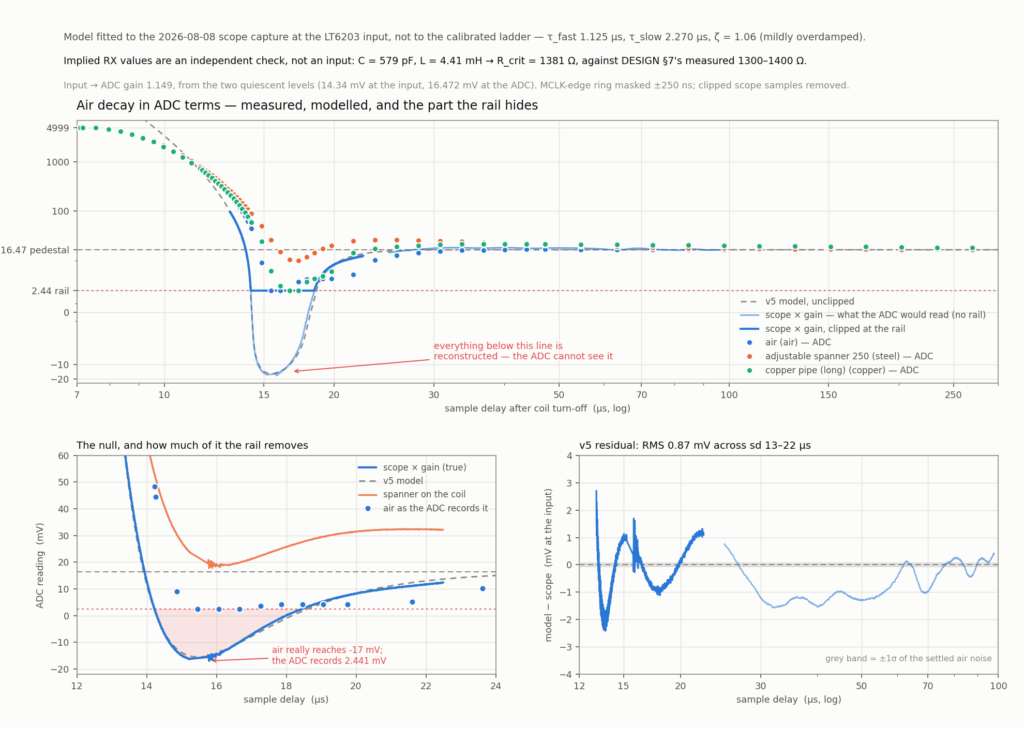
The last entry finished with me saying I’d have to put the scope on it, so I did — on the amplifier input this time, rather than reading the ADC and guessing at the rest. Going in there gets you the whole decay, including the part the converter never sees. It came out mildly over-damped rather than critically damped, which is what I’d been assuming for months, and it crosses zero exactly once, just as Claude said last time. Nice to have it measured rather than asserted.
Which brings me to the interesting bit. A few microseconds after turn-off, air dips negative for a while before settling. That null is real coil physics, not an amplifier artefact — it’s there before the amplifier, and it responds to metal. Put a steel spanner on the coil and the crossing goes away altogether. But my signal path is unipolar, so the whole dip happens underneath the floor and the ADC cant sample there.
I’d have called that a noise problem a month ago, and it isn’t. Everything I measure is target minus air. Where air has been clipped up onto the floor, the number I’m subtracting is too big, so the difference comes out too small — and by an amount that depends on how strong the target is. It never looks like an outlier. It just quietly shrinks things.
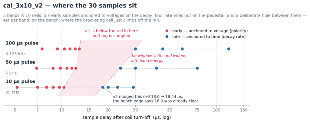
So the new profile has a hole in it: six early samples down the fast end, nothing at all through the null, then four late ones out where the last entry was looking. Three bands, 100, 50 and 10 µs, 30 channels where the old one had 63, so about double the sweep rate . It’s the first profile I’ve cut with a model in hand instead of sweeping and hoping. What I don’t much like about it is that the null does carry target signal, and I’ve thrown it away deliberately to get a clean corpus. If I end up wanting that region back I’ll have to deal with the clipping properly rather than stepping over it. In the meantime nothing I’ve already captured can come with me, so it’s yet another capture run from scratch.
13/8/2026 – Blown Regulator Brings New Hope (Who let out the smoke)
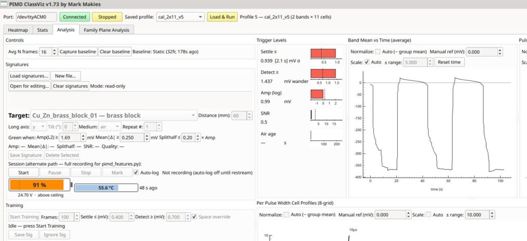
The +15 V regulator died in the middle of all this, and the replacement soon started doing the same
thing, dropping out and coming back every forty seconds or so. By using a higher proportion of 100us pulses I pushed the 7815 too far, much too far. Slowing it down fixed the problem, but adding a fan to the enclosure, nailed it.
I thought a fan so close would cause issues or noise however, the noise floor came down by about a quarter. Warm-up from cold used to be a fast drop followed by a long slow soak that was still creeping half an hour later; now it settles cleanly in about six minutes and lands in the same place every time. Another lesson learned: keep it cool, hot components drift a lot more than the battery drop I was chasing. Temp was quietly one of my biggest measurement variables all along.
The other loose end from last time is closed too, and it took one resistor. The dip under the floor
was never a noise problem, the signal path just couldn’t go low enough to see it, so a 240 k from
the 5 V reference into the amplifier input lifts everything about 100 mV clear of the bottom.
Nothing clips now, air included. The null I’d been carefully sampling around turns out to be the
best part of the whole ladder for telling steel from brass.