GeoCore started because I ended up with heaps of cardboard cores and I hate throwing anything out. The idea is dead simple: 3D print a set of colourful hub connectors, grab the cores, then snap everything together to build cubes, domes, bridges, geodesic frames, whatever.
But most importantly, I didn’t want to design each one myself and work out the geometry and maths, so I got AI to do it instead.
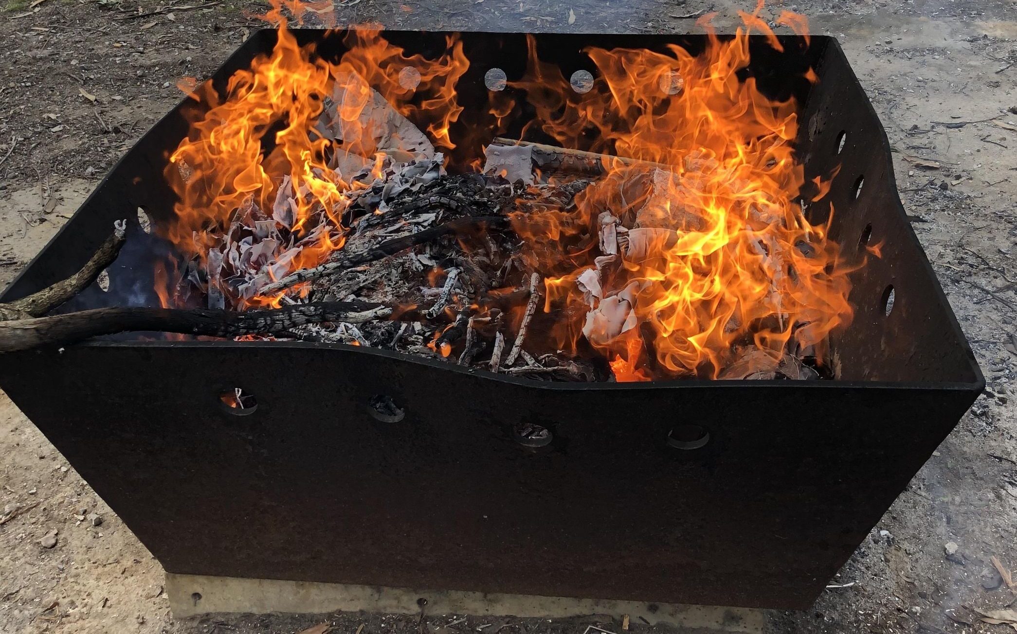
I built this fire pit back in 2018. I wanted something that was going to last and could take a bit of punishment, so I came up with a design on paper and got it laser-cut at my local steel supplier, Surdex. I went with 10mm plate.
I then undertook my biggest welding project to date, with minimal skills and budget equipment.
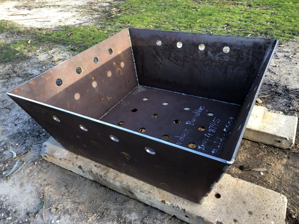
The result is a 1.2m square pit (at the top) that weighs a fair bit and takes a serious load of wood. It’s been through plenty of big burns since and shows no sign of giving up, aside from a bit of ‘character’ warping.
It sits on concrete blocks, with loose bricks plugging the ends underneath so I can open or close them to control airflow.
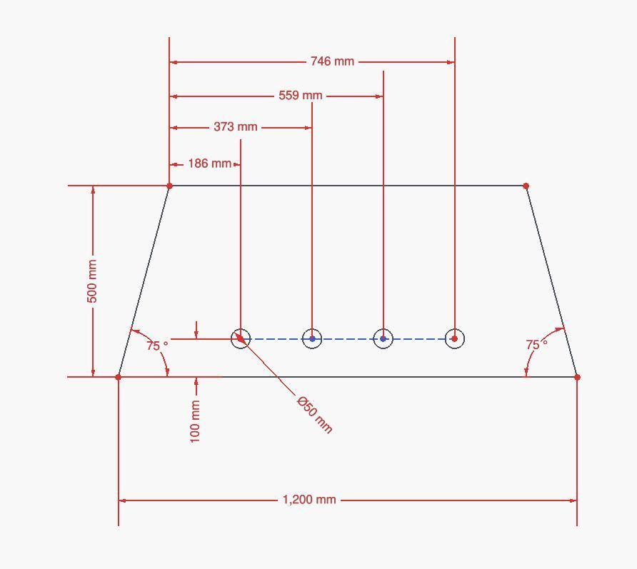
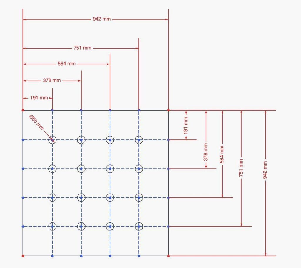
Dimensions:10 mm (3/8″) thick mild steel plate, 1200 mm (47″) opening at the top, 942 mm (37″) square base, 483 mm (19″) high.he shape, I’ve since learned, is an inverted frustum — basically a pyramid with the top chopped off.
Weight: The delivery docket says 287 kg (633 lb) of steel, but I never weighed it.
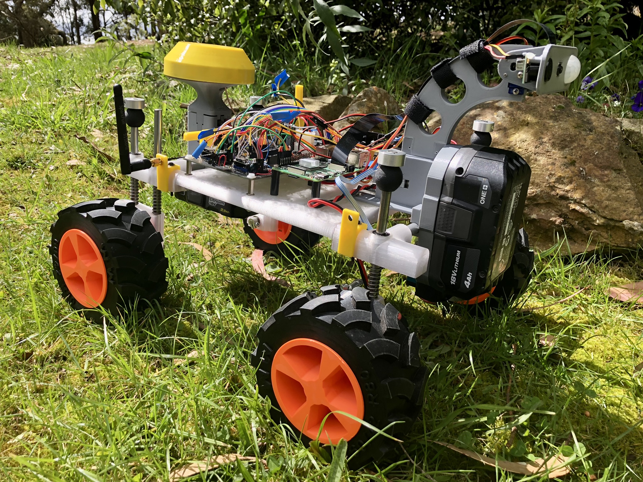
Roverling is an autonomous robotic vehicle capable of navigating via IMU and GPS, executing waypoint-based movement, dynamically adjusting steering and velocity using PID control, communicating via RC, LoRa, or Wi-Fi for remote or semi-autonomous operation, and logging telemetry for real-time monitoring and analysis.
It’s not the best design. It’s not refined. The code isn’t elegant. But it works – and it’s fast.
Want to build your own, or something similar: All design files, schematics, python code, 3d models and build tutorial all here for free.
A few months back I created a basic mobile platform using parts from an old 3D printer. It was fun but not very practical.
I designed Roverling Mark II so I could experiment with a practical, configurable, and reliable mobile platform. Hopefully, one day we get it to do some useful stuff around our bush block, like:
Searching paddocks for weeds and recording locations.
Navigating down a 200m drive to check if the gate is closed.
Navigating up the drive 50m to check that the machine shed roller doors are secure.
Recording animal sightings on the block. We’d see up to 50 ‘Roos’ per day on our block.
It would be good to identify and scare deer away from our olive grove.
And a friend already wants to mount a metal detector and do automatic scanning of a large area.
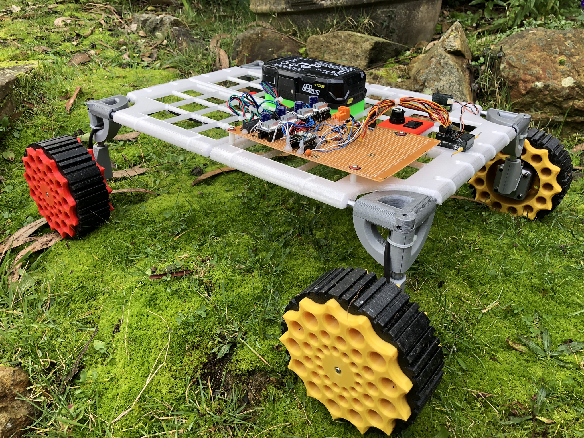
To that end, here is the complete design and everything you need to know to make your own or any variation. As much as possible I’ve kept the cost down to a minimum, reused some older parts, and printed as much as possible.
Specs:
440 mm long x 350 mm wide, 250 mm max height, 200 mm nominal platform height
3.5 kg without battery, uses an 18V power tool battery
Up to 22 satellite GNSS receivers, augmentation using SBAS, 1Hz updates
IMU: 3x accel, 3x gyro, magnetometer, pressure
2.4Ghz 6 channel RC receiver and decoder, with diverse receiver
2 channel motor quadrature decoders
2 channel motor current sensors (effectively torque sensors)
Sonar, ranger
915 Mhz LoRa module. Comms at 1800 bps, 64 byte telemetry packet, 16 byte command packet, encrypted, super reliable
LoRa base station, which is effectively my MQTT gateway for telemetry and commands back
Mapping module runs on desktop from the MQTT feed to produce real-time tracking info overlaid on an image (for me an old NearMap screenshot).
On board, RPi 4B w/ 4G running the latest OS with a camera 3 module. Work has just begun here, but object detection is working a treat, as does image capture and streaming.
All the 3D design is done in FreeCAD and all the slicing and printing on a Prusa platform. As well as the actual design files, I’ve also made available stl model files, g-code files, and Prusa project files for all parts.
The schematic is done with KiCAD. I used mixed prototyping methods and no PCB has been designed (yet) so you will need a fair understanding of how to layout and wire correctly.
All the code is in Python. I’ve pretty much written my own drivers for all of the low-level stuff except the sx1262 suite for LoRa. I’ve tried to document as much as possible.
BUILD TUTORIAL
Part 1: Mecha
Motors
Rather than steppers, I’ll be using brushed DC motors. Good ones, with planetary gears and optical encoders aren’t cheap, however, I have a few lying around from the 90s with suitable LM18200 H-bridges.
All of these were recovered from a SocBot platform, designed in 1999 by RMIT University to compete in the RoboCup games in Stockholm in 1999 and in Australia in July 2000.
This last SocBot has been lying around in storage since then and is starting to rust. It probably won’t make it into a museum, so parts it will become. The electronics are pretty old, a 68HC11 8-bit processor, running at 16MHz, programmed in assembly code, and a Xilinx 3000 series FPGA to achieve lower-level functions (kicker controls, quadrature decoder, PWM generation, etc). Now all of these are easily implemented on a $7.50 RP2040 MCU!
Back then these SocBots cost over $15k each to make.
The SocBot design was based on a 28.8V power supply (4x 7.2V NiCad RC racing packs), but there shouldn’t be an issue running at 18V, just less torque and speed. The SocBots were pretty heavy, at least 15kg, so if I can make this one lighter, the reduced voltage and subsequent torque shouldn’t be a problem for the acceleration I have in mind.
The motors I have recovered are Maxon 2332.909, 11W, 24V, diam 32mm, 17.83:1 planetary reduction with 100 CPT quadrature optical encoder. At 24V stall torque is 75 mNm * (18V/24V) * 17.83 ratio = 1003 or close enough to 1 Nm per motor at 18V – nice. The measured weight is 340g each.
Gear Specs (can’t find actual specs from 1999, but this is very similar): part number 166159
Hubs (1x front left, 1x front right, 2x rear)
Rather than a custom design for the motor mount, I have decided to use a more universal approach to make it easier for others to follow with different motors, given that they are the most expensive components.
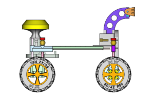
My particular gearhead matches one of the profiles on the ‘Motor Mounts For Andymark Neverest Motors – 1702 Series Quad Block Motor Mount ‘ (GB-1702-0032-0001) mounting bracket (shown in red below). So I designed my hub to suit, which should mean that the other motor mounts should also be compatible with this hub, as long as the motor diameter is less than 32mm.
In the next pictures, steering components are described later.
Rear Hub
A simple printed piece with two 6x15x5 bearings, and attached to the suspension/frame with two 8×150 SS rods.
Tyres & Wheels
I’m making these tyres with a greater section profile, less infill, and less perimeters compared to version 1. I also designed, I think, a better tread profile, which also requires less support material to print.
In the wheels, I have included a captured nut and set screw so that it is easier to secure to the motor’s D-shaft.
The front wheels have more space on the inner side to fit the motor, whereas the back wheels have an extended collar.
Right and left tyres are a mirror image of each other, achieved at the slicing stage, rather than with FreeCAD. Fit the tyres so the ‘arrows’ on the tread point to the main direction of travel.
Steering
I’m not sure if it’s a done thing, but I used the constraint-based sketcher in FreeCAD to dynamically simulate movement in the design. You basically set up all the constraints but don’t fully constrain them. I then drag the linkages around and see the effect. This allowed me to simulate many different design variations before committing to anything. It’s not a perfect tool, but for what it costs it can do amazing things.
I’ve left the simulation ‘part’ in the FreeCAD project, so take a look if you want.
Rather than trying to reinvent from scratch and fail, I’ve decided upon a proven Ackerman Steering Geometry with the following characteristics:
Kingpin centres: 200 mm x 300 mm
Steering rod to kingpin centre length: 35 mm
Tie rod length 177.3 mm for about a 0.5-degree toe-in on each side
Ackerman angle 18.44 degrees
No camber or caster angle at this stage.
Linkages aft of the wheel, initial designs had it forward.
I’ll be using a standard-size RC servo to control the steering, but rather than use this to linearly move the steering rod, I’ll mount it to one wheel hub so it effectively fixes the angle between the steering rod and tie rod. Between 60 – 180 degrees gives full steering in both directions. The servo I have at hand is rated at 0.3 Nm (3 kg.cm) which can easily be replaced with a 1 Nm unit if required.
The front left hub also serves as the mounting point for the servo, with the shaft output directly in line with the calculated Ackerman geometry.
Important note: I have used the normal left/right car-based nomenclature to identify the sides. This is NOT consistent with that used in FreeCAD, as it is based on looking from the outside of the object rather than from within.
Suspension
Independent. A very simple sliding pillar design. Each hub has one or two 8mm vertical SS rods securely fastened to the hubs. The front ones are effectively the kingpins.
Then starting from the bottom working up:
Printed hub
Steel shim 8x11x1
2x Stainless Springs 1x10x40
Steel shim 8x11x1
Linear Bearing 8x15x24 – embedded in chassis corner
Steel shim 8x11x1
Printed Flex Stop
Clamping Collar 8x21x9
Pics show unloaded and with a 10kg payload.
Chassis
In my last design, I used 8mm steel rods that added significant weight. This one uses a plain old 10 x 1.5 mm aluminium rod.
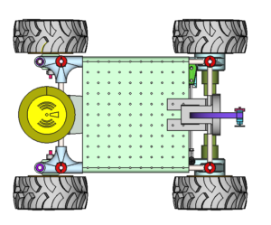
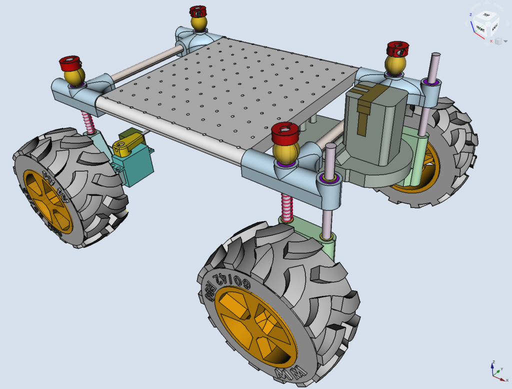
The corners contain the linear bearings and affix to the axial and radial aluminium rods. The design allows me to extend the platform on the front for sensors whilst using the back to secure the battery pack to help distribute the weight.
There is a generic platform with holes on 20mm centres for mounting electronics and other accessories.
In the pictures, you will also see my battery adapter, which has been modified from the previous design to fit this chassis.
Model
Print Parts
I usually print with generic brand 3D filaments and until now I haven’t really had a problem with them. In this picture, the black parts are Bilby 3D brand PETG, the clear is eSun PETG and all the other colours are Bilby 3D PLA. The black stuff is very brittle, more so than any of the PLA’s.
Moving forward this entire project will be printed in eSun branded filament as I have had much success with this brand. I have no commercial association with eSun.
In the sliced project and G-code file names, Rn denotes the revision number (n) of the slicing and printing attempt, not the design revision. So R205-Hub-FL-R3.3mf means Roverling design version 205, of the Front Left Hub, and Revision 3 of the slicing and printing parameters.
Support: make lighter and further separation. It is very easy to remove, just grab it from the centre and pull it off quickly – like a bandaid.
And importantly, limit the maximum volumetric speed to 3.5mm^3/s On the i3 Prusa I used the provided SemiFlex profile, but increased the volumetric speed by around three-fold without printing issues. About the only change I make to the printer is to loosen the feed pressure screw substantially.
There is also a ‘tyre label’, which I merge with the main tyre to provide the writing.
Within the slicer, I have mirrored two of the prints for the opposite side. Mainly to ensure that the bottom/top of the print is the same on each side and the writing is on the same side. Not entirely necessary.
Inside the tyre is nearly all air, only 3% infill to hold up the top
2x Front Wheels R2 & 2x Rear Wheels R1
Material: eSun PETG in solid orange
Generic setting: 0.3mm draft
Perimeters: top: 4, bottom: 3, perimeters: 5
Infill: 20% grid
Avoid perimeter crossing
Top/bottom fill pattern: concentric
Generate support material everywhere
Note that one of two runs might be left hanging to the top rim edge. Just chop them off as nobody will see anyway. It’s not worth creating support just for this.
Don’t fit the tyres to the wheels yet
1x FL Hub R3 & 1x FR Hub R2 & 2x Rear Hub R1
Material: eSun PETG natural
Generic setting: 0.3mm draft
Perimeters: top: 5, bottom: 5, perimeters: 6
Infill: 10% rectilinear
Top/bottom fill pattern: concentric
Generate support material everywhere
Don’t attach anything yet.
2 x Front Chassis Corners R5, 1 x Back Right & 1x Back Left (mirror) Chassis Corners R2
Chassis Corners. These were very strong in the last design as the fill was 100%. This also made them heavy. The new design aims for about a 1.5 mm wall thickness with minimum infill.
Material: eSun PETG natural
Generic setting: 0.3mm draft
Perimeters: Top: 6, bottom: 5, perimeters: 6
Infill: 10% rectilinear
Top/bottom fill pattern: rectilinear
Then carefully clean up the supporting material. Don’t drill out 10mm holes, just use a 9.5mm drill, by hand, to remove support material.
The rods need to fit very tightly – you will need a hammer to get them in, BUT NO MORE than 30mm. And then a pair of pliers to get them out – twist and turn as you go. Same with linear bearings. But don’t do this step now. Once in they should stay in.
1 x Platform R2
Hard to stick down at the edges at bed 80 degrees, so up to 90+ degrees and slow the first layer down to 80%
Material: eSun PETG natural
Generic setting: 0.3mm draft
Perimeters: Top: 4, bottom: 3, perimeters: 8
Infill: 20% grid
Top/bottom fill pattern: monotonic
Generate support material
4x Flex Stop R1 (shock absorber)
Material: eSun eLASTIC Flexible TPE in black
Generic setting: 0.3mm draft, no special settings, no support
Limit maximum volumetric speed to 3.5mm^3/s
1 x Servo Horn Adapter R2
Material: eSun PETG natural
Generic setting: 0.3mm draft
Perimeters: top: 8, bottom: 8, perimeters: 6
Infill: 100% rectilinear grid
Top/bottom fill pattern: monotonic
Generate support material
1 x Battery Carrier R1
Material: eSun PETG in silver (looks grey to me)
Generic setting: 0.3mm draft
Perimeters: top: 4, bottom: 4, perimeters: 4
Infill: 20% grid
Top/bottom fill pattern: monotonic
Generate support material everywhere
Procure Parts:
I have no commercial affiliation with any of my suppliers. If there is a link it’s just where I got mine from.
No particular order has been formulated, as I’ve rebuilt and remade a few times. Below are some of my recommendations & techniques. Otherwise, I hope the pictures tell a thousand words.
Chassis
Chassis first. Linear bearings into corners, line up, and use a vice. It MUST be aligned otherwise you’ll break something.
Make sure the 10mm holes are very clear. The aluminium rods get hammered in – support well and ensure proper alignment. But don’t do them yet.
Platform first as it is very tight. Bang the side rails in from the end, protecting the metal, until they protrude evenly from both sides.
Then assemble to short edges, using the installed platform rods as a size guide. I used a hammer to press them in but a vice or clamp might be better.
If you are going to use my battery adapter, you need to install this first on the rear rod.
Then press the small assemblies onto the platform section and voilà. Centres need to be accurate (200 x 300 mm).
I drilled extra holes and used M3 x 30 CS bolts to prevent rods from turning and twisting the platform, just in case.
Wheels
Install M4 x 7 square nut after drilling out hole to 4.5mm
Method for front and back wheels:
Method for back wheels:
Put together the rear hub assemblies, referring to the pictures in the Hub section. Attach rear wheels to the hub through bearing and shim and lock in place with a collar.
For the front assemblies carefully press motor shafts into the front wheels. I used the hub for leverage.
Tighten all 4 shaft locking screws
Fit all 4 hubs to corner brackets, using shim, spring/s, and shim, then pass through the linear bearing, shim, flex stop, and finally locking collar.
Next tyres. Use a small screwdriver as a tyre lever, but don’t press too hard on the thin wheel rim, instead leverage from the middle where damage won’t be seen. The locking nut should almost be flush, so the flex will slip over it.
Steering Components
And finally the steering components. Again check previous pictures for the servo horn adapter, threaded rod and ball linkage arrangement. Don’t do tyres first as you may damage the steering.
That’s the assembly complete, except for these last-minute fixes. A larger steering servo requires this section to be sliced off. Also need a redesigned servo horn.
Camera Bracket/Mount
The camera and sensor tilt head was a later addition.
Part 2: Electronics
This is probably the least documented section. I started with a list of actual IOs that I think I needed and then split these logically. I ended up with an RP2040 processor for motor control, motor sensing, steering control, and an RC interface. This can, at the lowest level, run independently, using the RC just as a remote control.
The second RP2040 handles the telemetry, comms, and all the other peripherals.
Made from an old film tin lid, 100 mm in diameter, a printed cover, and a base that also forms the battery adaptor clip. Also serves as a good place to hide the extra cable length.
PLA is fine, nothing special is required, just the basic 0.3 mm draft template. You will need support for the base/battery clip combo to hide the cable.
The tin is easy to solder (ground plane connection) but you must protect the cable from the sharp edges. I use hot glue, lots.
RC Receivers
A plastic holder protects the wires from breaking and the receiver plugs into these female sockets.
Breaking Out More RP2040-Zero Pins
Wiring
LoRa Base Station & MQTT Gateway
If you are using a Pico W, be warned that mounting it as designed (one on top of the other) brings the RC cans/components too close together. This will result in between a 10 to 20 dB drop in receiving SNR as you start to go below -70 dBi RSSI.
You’ve been told – it took many days to figure this out.
Part 3: Code
There are multiple Python modules that need to be loaded into the three RP2040s. Everything you need to know is on my GitHub as is all the code for you to download.
Basic block diagram
Motion Processor
Works independently of other modules. Can use RC to control without any other modules. On RC toggle FLAPS to put it into RC mode. The onboard LED will change from steady green to flashing pink. Ensure throttle is at min first. Ailerons control steering, elevator controls camera tilt. GEAR puts it into reverse mode.
Provides a gateway for Roverling LoRa commands and telemetry to MQTT message broker over WiFi. The onboard LED flashes blue when commands are received. A single message is delivered twice a second and looks a lot like this. (On MQTT Explorer): (3172, ‘-37.0000000, 144.0000000’, 1, 4, 3.0, 640.4, 0.0, 0.0, 0.039, 0.043, 0, 0, 10, 50, 51, 51, 9, 10, 0.013, -0.037, 1.015, 0, 0, 0, 0.034, -0.037, 0.455, 19.734, 944.5, 10.25, -42.0, 384, 0, 0, 0, 11.0, -45.0)
Roverling was designed so that code development can take place without providing any external power. The USB-C connection to either processor for download, test, and dev, is enough to power everything on board, except motors, including the RPi4, surprisingly.
I use this all the time and use the onboard power switch to fully power when I want to drive the motors. This system has allowed for very rapid development. The GUI will show a dangerously low battery voltage, just ignore this.
Gateway Board
The Roverling telemetry base station now has a printed enclosure. Communication with Roverling MkII is good for up to 500m, and appears to show no problems in denser bush or terrain.
The base station is just a gateway between the Long Range 915MHz spread-spectrum communication systems and my home MQTT messaging service. The Roverling telemetry rate is limited to 1800bps, but within a small 64 byte encrypted packet (200ms Tx time, every 500 ms) we manage to fit:
GPS time stamp, latitude, longitude, GNSS quality, number of satellites, accuracy, altitude, left & right velocity, left & right motor current/torque, left & right motor power (PWM), remote control receiver – 6 decoded channels, acceleration on 3 axis, rotational sensor / gyro on 3 axis, magnetometer on 3 axis, air temperature & pressure.
Communication is good for 500+ meters line of site. With Roverling inside a large metal shed, and the base station 80m away inside and at the back of a timber structure, we get around -105dBm RSSI and an SNR of around -3dB.
This same MQTT service over WiFi is used for remote monitoring and control of multiple systems around our property, including water levels, pumps, outdoor lighting control, irrigation, gate status, environmentals, etc, etc. Some of these systems are based on 433MHz MQTT gateways I developed years ago that I was going to migrate to LoRa, but they are still working well using my own protocols.
Gateway module in a nicer looking enclosure
Part 4: GUI
I used VS Code to develop and run these python modules in a virtual environment. Programming is not my strength, and nothing has been packaged properly, but all my code is here.
Gateway < — (MQTT over TCP via WIFi) — > Desktop Computer (GUI)
You need to have Wi-Fi and MQTT broker infrastructure already in place to use this solution. You could also remix the gateway to provide any other kind of communication channel/protocol. You can also use any MQTT-enabled device. I use an app called IOT ON/OFF on my iPad and iPhone and use MQTT Explorer on my Linux desktop.
I use Mosquitto, an open-source MQTT broker, that runs on an RPi4 which also provides all the network services I need around here.
It’s all coded in Python using the Qt framework, on Xubuntu, I installed using: pip install pyside6.
The GUI graphics were designed in using pyside6-designer and compiled into Python with pyside6-uic.
MQTT Explorer worked great for development. In the below screenshot, each parameter was conveyed by a different MQTT topic. This proved problematic in the Qt / MQTT framework, so now there is a single topic that returns a string with ALL parameters.
GUI Elements
COMMS
Click on RUNNING/STOP to process MQTT packets Pkt count shows the number of packets received GPS Sec shows GPS minutes/seconds past the hour SNR and RSSI displayed for both ends
SYSTEM
Shows the approximate battery charge level, PIR status, sonar range, and 16 status bits.
RECORD
Click Paused / Recording to toggle a recording. Very simply, all received packets are saved to a CSV file that can be played back as if telemetry is being received live, except that you can change the speed.
LOCOMOTION
Displays velocity (not yet calibrated), current (same as torque and will be used to detect slip or stall in the future), and applied power. At the moment power is controlled only by RC channel 1. Soon I’ll write a proper PID controller with velocity and max acceleration as the input parameters. Negative velocity is shown when reversing.
IMU
Show processed data. Heading based on X & Y magnetometer Pitch and roll based on X, Y, and Z components of the accelerometer Temp, pressure, and calculated altitude based on pressure & temp X & Y magnetic flux components, current limits, and new ranges for calibration
This picture shows the result of slow rotation about the centre, followed by a quick direction change. X and Y axes represent the respective magnetic fields.
Magnetometer calibration
The first few seconds of the video below show the X & Y components of the Earth’s magnetic field as the Roverling is slowly rotated around on an office chair. It’s pretty round but has a little distortion due to the magnet in the GPS antenna which is about 150mm away.
The last half of the video shows the fields whilst the Roverling is outside moving around, as per the previous post. I carefully twisted all current-carrying wires with their return to prevent EMI from impacting the magnetometer additionally, the Roverling was moved manually rather than on its own power, so there shouldn’t be too much EMI generated due to motor currents. The chart clearly shows field strength almost doubling in some locations. There is a big spike as I travel around a power pole and others that I’m unsure about. My calibration is good enough for now and could probably be further enhanced using GPS positional deltas to calculate heading.
Also used this – sometimes the old ways are the best.
GPS
Pretty much everything out of the $GPGGA sentence.
Below GPS data are the tools to set the origin of the aerial photo. You’ll need to modify the code (add your own photo/map), put GUI into record mode, and drive around, as much as possible visiting accurate positions you can see on the map. Then adjust the bottom left coordinates and scaling factor.
Yellow points on the graph indicate that quality = 1, and red means we had quality = 2
You may also notice the GPS variance chart. This was created to observe variance/error when NOT moving. It really needs to sit outside in the open sky for about 5-10 minutes, and at that point, the divergence is usually less than 30cm. Interestingly the GPS quality number (1 or 2) or the reported accuracy doesn’t appear to have any correlation with the actual accuracy/divergence that I measure.
GPS Test
What you see here is a sped up 3 minute tour to test the Roverling Mk.II GPS solution. You’ll notice no velocity registered on GUI as I took the Roverling around on the ride-on mower.
What I found more important is the number of satellites in view. I found at my location I need at least 15+ to achieve a variance of less than 0.5m, but I usually get 19 and at most 22. For this run, you will notice that I managed 19-20 sats, even under trees.
Roverling MkII GPS Test
RC
Shows details of all 6 channels. Channel 6 > 75% puts the Locomotion Processor into RC control mode, shown by this panel changing to light blue. Ensure CH1, throttle, is at minimum before toggling gear (ch6) switch – otherwise, Roverling may shoot off the desk! Happened to me more than once whilst developing.
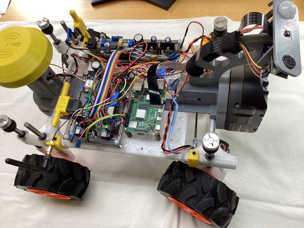
Part 5: Raspberry Pi
Raspberry Pi 4B 4GB w/ 64 GB SD Flashed with most recent 32-bit Raspberry Pi OS w/ desktop (3/5/23) Raspberry Pi Camera Module 3
I played around with object recognition, face recognition, video streaming (UDP & TCP), and video capture and save. A few examples are below.
This video demonstrates the problems navigating, even manually, with an un-stabilized camera and very basic suspension on a gravel road.
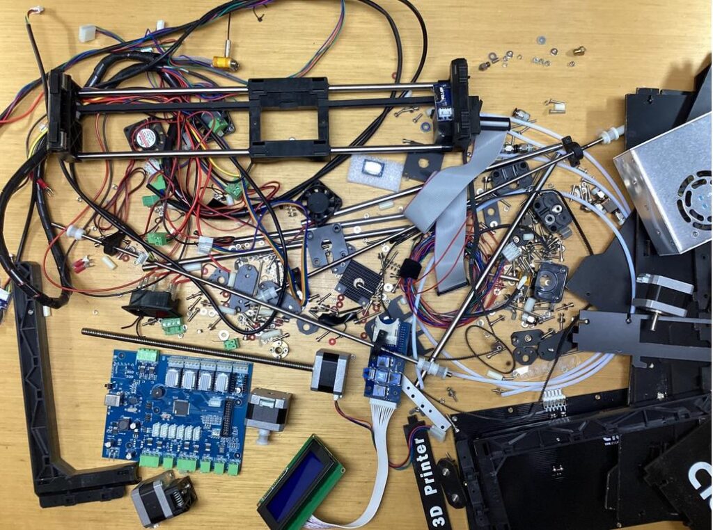
Made almost entirely from my old 3D printer parts + parts printed with my new Prusa printer.
My first 3D printer was a CTC generation 2 clone of MakerBot ‘The Replicator Dual’, circa 2012. It died a little while back and has since been replaced with a Prusa i3 MK3S+. Not one to waste any bits, I disassembled / broke down the 3D printer into component pieces, looking for inspiration for a project – one made mainly from these bits.
And I came up with the Roverling. I’m attempting to make a wheeled platform, mainly from these bits, that can be used in a multitasking environment and for further development. I’m designing and making it on the fly so I don’t have an overall picture or plan.
The basic design consists of 4 independently driven wheels using stepper motors. The plan is to use differential drive to manoeuver and steer (untested). I would use servos for steering, except I’m trying to use just what’s available as much as possible.
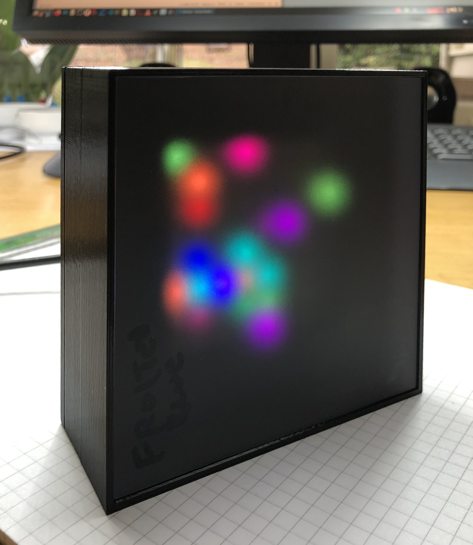
I wanted to make something artistic and dynamic using an 8×8 matrix of RGB LED’s, that I recently discovered.
I used a cheap RP2040 MCU module, programmed in Python to produce the random patterns. I just played around with numbers and algorithms until I liked the look of them. It seems that people all have very differing favorites and some that I didn’t like, others love. So to that end, I created 4 different algorithms which create distinctive patterns over time. I didn’t want to use any switches so an accelerometer determines the orientation of the cube which sets the mode. The unit resets itself when put on its back.
The Cuboid was used to make some colourful videos and also inspired the Glyph Generator project.
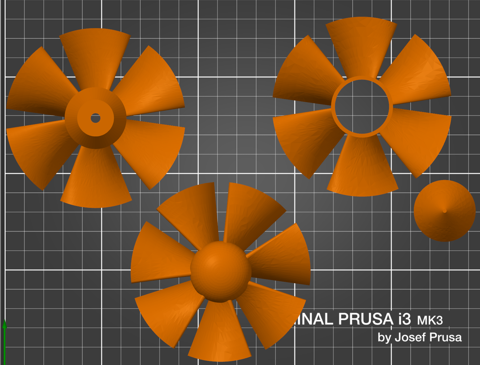
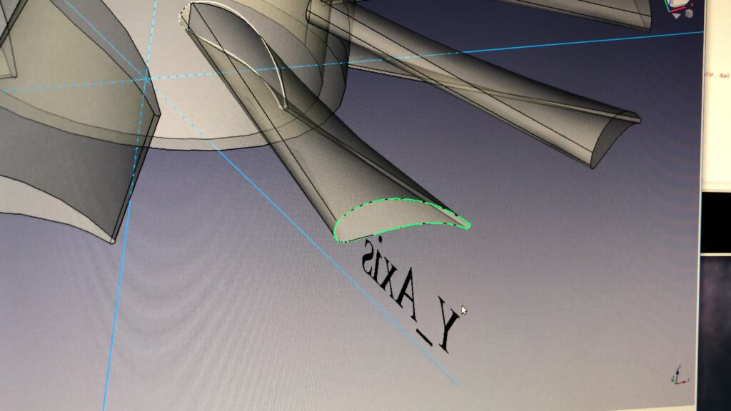
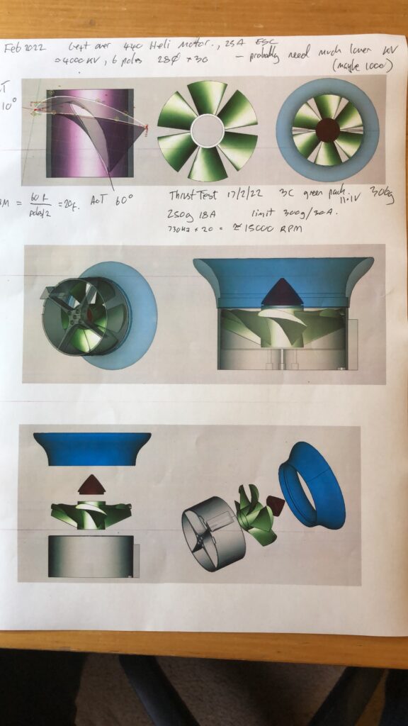
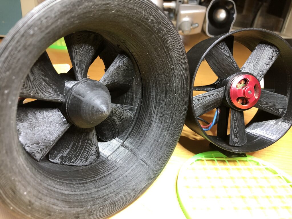
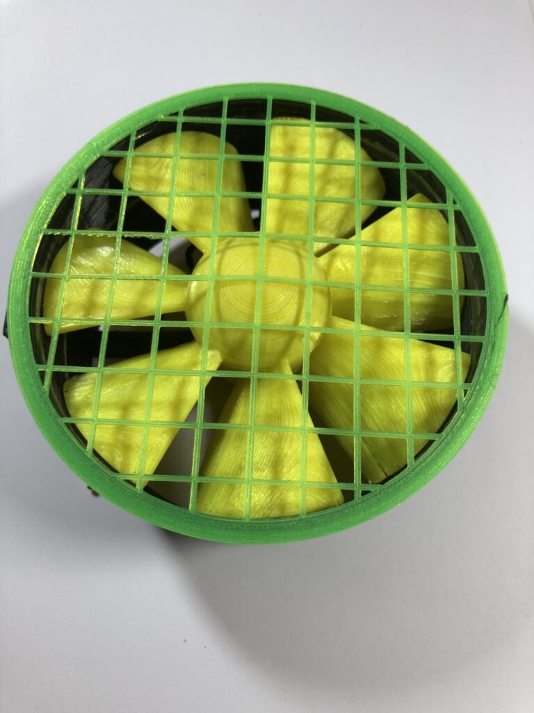
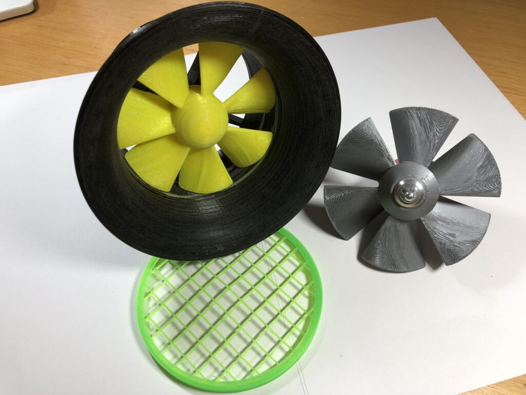
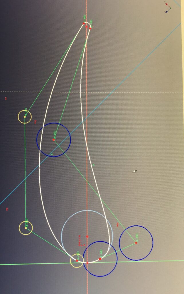
I had some spare BLDC RC motors lying around – rated at 4000Kv, 6 pole, 24mm diameter, 30mm long and I wanted to design my own EDF (Electric Ducted Fan) for use in a VTOT (Vertical Take Off Thing).
As it turns out it belw lots of air but not enough to lift itself and the battery. In any case I published my 3D propeller designs and they were a bit of a hot. Not sure if anyone actually printed and used them though.
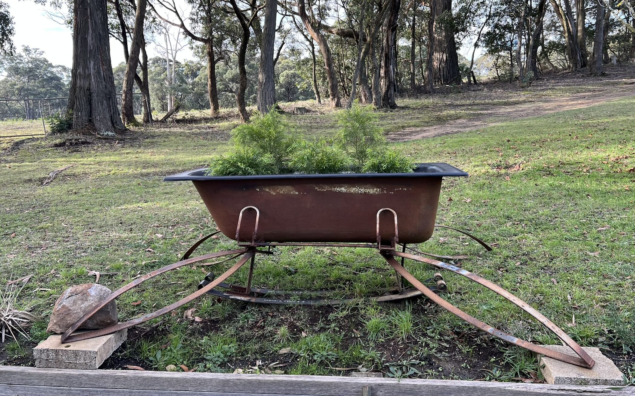
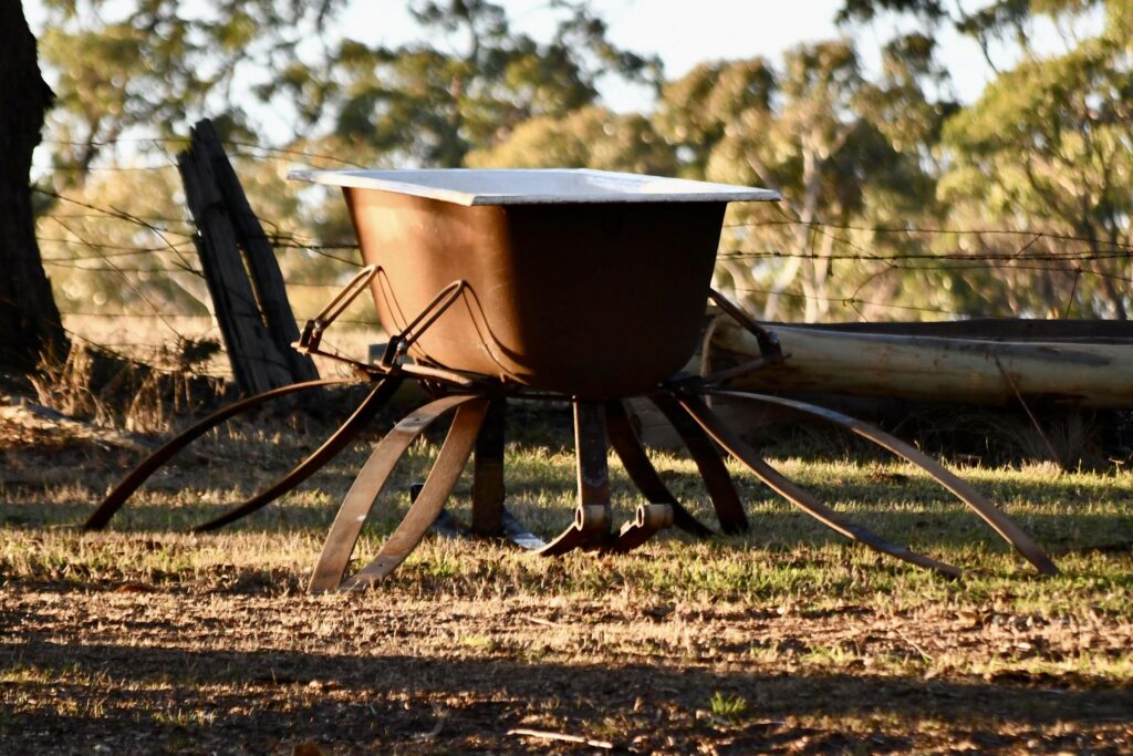
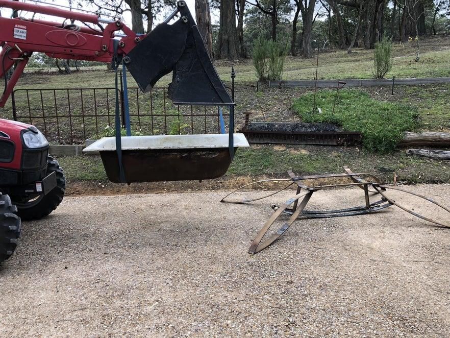
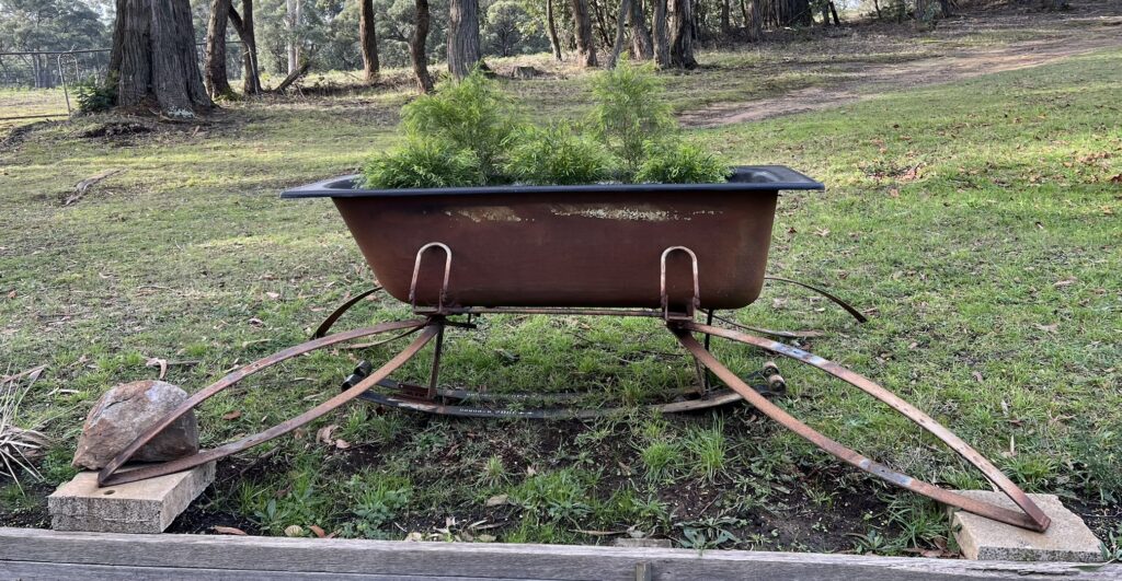
A neighbour upgraded his Land Cruiser suspension and I ended up with the old leaf springs. We’d also had a cast iron bath sitting in the bush since we moved here two decades ago, that I’ve been meaning to do something with.
I’m not a professional welder, but I reckon I’ve picked up enough over the years to try a project like this.
I had a vague idea it might become an outdoor bath, but once the frame was done it was clearly too big and awkward, so I never tried. With encouragement from my wife, it is now a large planter, with irrigation pipe routed up through the drain hole.
This is not a complete or ready to build project – yet. These pages are a blog of the design process – what went wrong, the dead ends, what went right, and the things I never quite figured out.
1/11/23 Let’s Build a Metal Detector with no Previous Experience
There are heaps of designs and tutorials out there that have given me some great ideas, but as always, I like to start from scratch and design and build a solution to suit me. Although I prefer the digital domain and Python, it’s not going to be fast enough. The maximum sampling I’ve been able to achieve is 50 kHz, or about 20 µs, on an RP2040 running Python. Nowhere near quick enough. I need sub-microsecond samples to make this work, so I’m going to have to do a bit of analogue mixed-signal design.
The basic premise is to capture decaying pulse waveform levels at very specific times: the first one between 1–5 µs after the pulse is removed, and the next between 5–50 µs. Accuracy is absolutely key, so all analogue components will be used up to the sample-and-hold chip (300 ns capture, 100 µs hold). After that, an interrupt will trigger the slower RP2040 ADC reads, which will then store the data sample, synchronised with the GPS position, along with a small telemetry packet to ensure Roverling stays ‘on-mission.’ I’ll probably aim for 10k samples per second.
First step, though, is to replace my now-broken cathode ray oscilloscope—it has served me well for many decades. I’ve even got the original brochure. I tried, but it’s just not possible to properly design and tune this system without being able to see what’s happening at a 100 ns resolution. Luckily, my HP1630G logic and state analyser from the same era still works well, although it only samples at 100 MHz.
And it’s time to read some literature, especially since I’ve never even owned a metal detector. The following references were invaluable in this endeavour:
Inside the Metal Detector by George Overton & Carl Moreland
Hammerhead Pulse Induction Metal Detector by Carl Moreland
Making a Fast Pulse Induction Mono Coil by Joseph J. Rogowski
Coil Basics by Carl Moreland
Designing Gain and Offset in Thirty Seconds by Bruce Carter (Texas Instruments SLOA097)
Op Amps For Everyone by Ron Mancini (Texas Instruments SLOD006B)
16/11/23 New Oscilloscope
Christmas has come early—out with the old, in with the new. These old bits of kit have served me well for decades, but it’s time to move on. Thanks to EmonaInstruments for the great service and almost instant delivery. I wish I’d had one of these 30 years ago when I was teaching undergrads about metastability—it would have been much easier than trying to adjust the phosphor persistence on a cathode ray oscilloscope.
Next, I’d better download and read the manual.
22/11/23 Design and Construct a Coil
Finally, all my bits are here, so let’s start building a search coil (v2). It’s 400 mm in diameter and constructed from four printed parts that are simply glued together. The inner race has 50 turns of 0.25 mm Teflon-coated silver/copper wire (wire-wrap wire) with an aluminium foil Faraday shield (no loop). This is the receiver and has a DC resistance of 20.1 ohms.
Over the top of the Faraday cage are 20 turns of 0.5 mm enamel-coated magnet wire, with a DC resistance of 2.1 ohms, which forms the pulse transmitter. Then, over the top of that is plenty of Kapton polyimide tape. It looks great on space missions, so why not use it here? (Plus, I no longer need it for holding down ABS prints.)
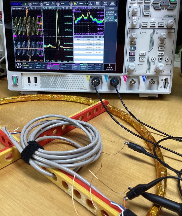
The next step will be to determine the critical damping requirements for both coils. To that end, I connected the (new) oscilloscope probes to the ends, expecting a 50 Hz signal, but that’s not what I saw. On the scope’s centre window, you can see the spectrum analysis, and that huge spike in the middle? Both coils are picking up something at exactly 118.75 kHz.
You can’t see it in this picture, but about 0.5 m away is my old monitor, which turned out to be fully responsible for this artefact.
Just goes to show that I’ll need an electromagnetically quiet place for calibration and testing.
6/11/23 First Coil – Working?
Analogue design is not my strong point, especially when it comes to inductors, but I’ve finally achieved some fantastic results with the coils. Firstly, I needed to create a bipolar totem-pole gate driver for the MOSFET. The parasitic capacitance can’t be overlooked if you want high-speed, non-linear FET switching. I used CircuitLab for the first time to simulate the circuit and was very happy with how quickly I could create the schematic and perform DC and AC analysis. This was critical in my choice of components for the totem-pole, though it wasn’t very useful for coil simulation.
The TX coil pulse is driven by a 100 Hz PWM output from the RP2040, with a duty cycle of 2^16 – 34 at 100Hz, giving a negative pulse of 5 µs. The TX coil needs to be critically damped to prevent unwanted ringing on the RX coil, which I achieved with a 220-ohm resistor. A maximum current of 10 A is realised within the first 1 µs, which suggests this should be the turn-off time. However, I’ve found much better results with a 5 µs pulse at the RX end, with diminishing returns beyond that.
The RX coil is not damped, as I couldn’t see any need for it on my oscilloscope, even though theory might suggest otherwise. The RX output is clipped in both directions using two 1N4148 diodes.
If you look carefully at my computer monitor, you’ll see the aqua (persistent) plot. The top of the envelope indicates no metal, while the bottom of the envelope shows its presence. Without any amplification, the difference is in the order of 500 mV within the 10–50 µs decay time frame.
I couldn’t have hoped for more at this stage.
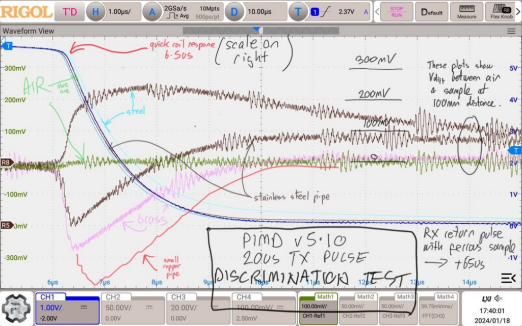
28/11/23 Wrong Coil Design
Most of the research I’ve done up to this point suggests using a short pulse width, with most sampling occurring in the 5–25 µs decay time frame. However, for my coils, this didn’t seem to provide the large voltage detection swing I was hoping for on the RX coil.
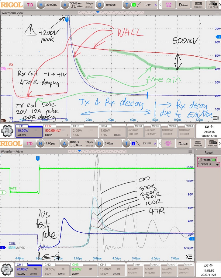
If I drive 10 A through 2 ohms for 50 µs, I get a much better result. The top chart shows the difference in RX coil voltage between free air and a wall with foil sarking. At about 40 µs after the impulse, there’s a massive difference, reaching 500 mV within another 60 µs. Interestingly, there are also detectable changes in the TX coil from 0–80 µs after impulse removal, as well as another change on the RX coil 5 µs into the pulse itself.
There’s a lot of useful information here, but the next step is to test with real dirt and real objects at various depths. I’ll then determine what voltage levels and/or sample time frames to use. Some machine learning could be really useful here. I’d also read that using only an 8-bit ADC wouldn’t provide usable data, but now I’m not so sure. Let’s first see what the RP2040 can achieve before complicating things further.
The bottom chart shows earlier damping tests of the TX coil. This resulted in selecting a 200-ohm damping resistor for the TX coil; HOWEVER, I had to reduce this to 100 ohms to also critically damp the RX coil. I then added specific damping to the RX coil only, which ended up being 470 ohms. Since they effectively form a tuned circuit, I used potentiometers on both until I achieved the desired waveform. Without first tuning (and ensuring your 10x probes are properly compensated), there’s no hope of obtaining the results shown in the top chart.
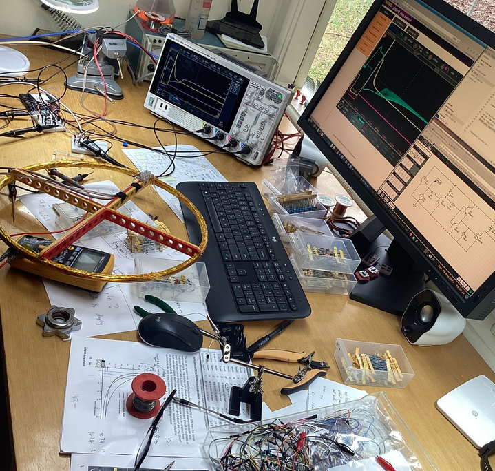
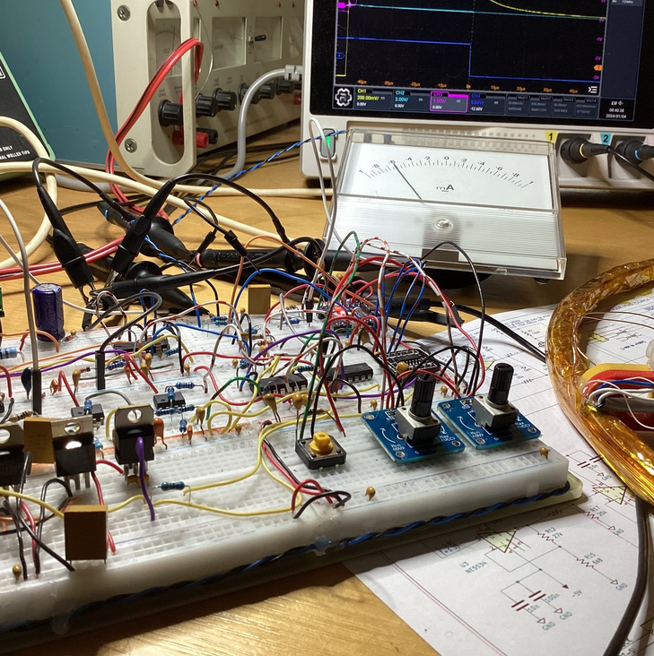
12/12/23 Getting the Hang of Op-Amps
Prototype 1 is complete—but a failure. It can detect a large object at 100 cm, but small close objects go undetected. The biggest mistake? Observing waveforms through ‘rose-coloured glasses’ using all the filtering, smoothing, and analysis capabilities of my new Rigol scope. When switching to high resolution at 2 GS/s and 16 bits, a different story emerges: one filled with noise that completely swamps the signals I’m looking for. Using a long display persistence highlights the problem areas even more clearly.
Now, I’m working on attempt #2 with a much better understanding of op amps. If you’re a rusty engineer like me, you can’t go past Op Amps For Everyone, a Texas Instruments design reference guide (SLOD006B). It’s a tough read but pointed me in the right direction.
The TX coil only becomes fully saturated at about 200–250 µs, so I’m now driving it for exactly 200 µs, resulting in a peak coil current of around 4.5 A. After the RX coil output is clipped to ±1 V, it passes through an NE5534 op amp (primarily an audio op amp) based preamplifier with a gain of 10 and an LPF set at 180 kHz. Next, it passes through another NE5534 with a gain of 13, giving the system an overall transfer function of 30 to 80 mV input maps to -3.3 V to +3.3 V output.
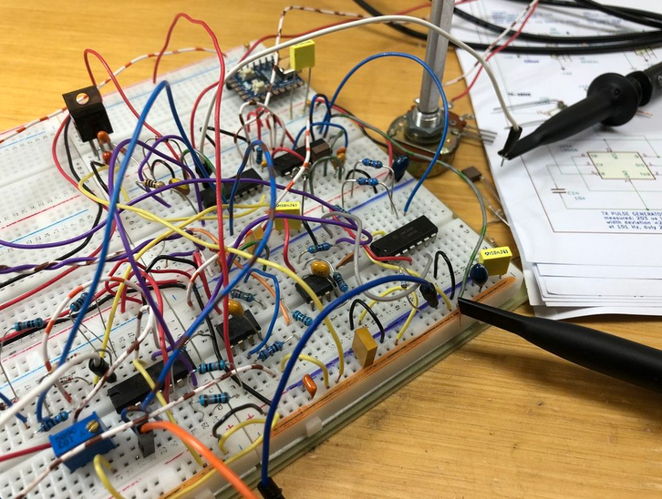
At 60 µs after the end of the TX pulse (but measured on the RX coil), a CD4066-based CMOS switch samples and holds the voltage.
This region (55–65 µs) provides the best signal-to-noise ratio. Sampling earlier than 55 µs results in poorer differentiation, while sampling later than 65 µs falls into the noise floor. Bench testing looks very promising—small objects are now easily detected, noise is largely gone, response time is quick, and I’m getting a clean and held voltage in the range of -3.3 V to +3.3 V. And all of this is working on a solderless breadboard!
The next step is to route this signal into an ADC (after attenuation and level shifting) and bring it back into the digital domain, where I’m most comfortable, for further development.
12/12/23 Learning (but in hindsight looking in the wrong area)
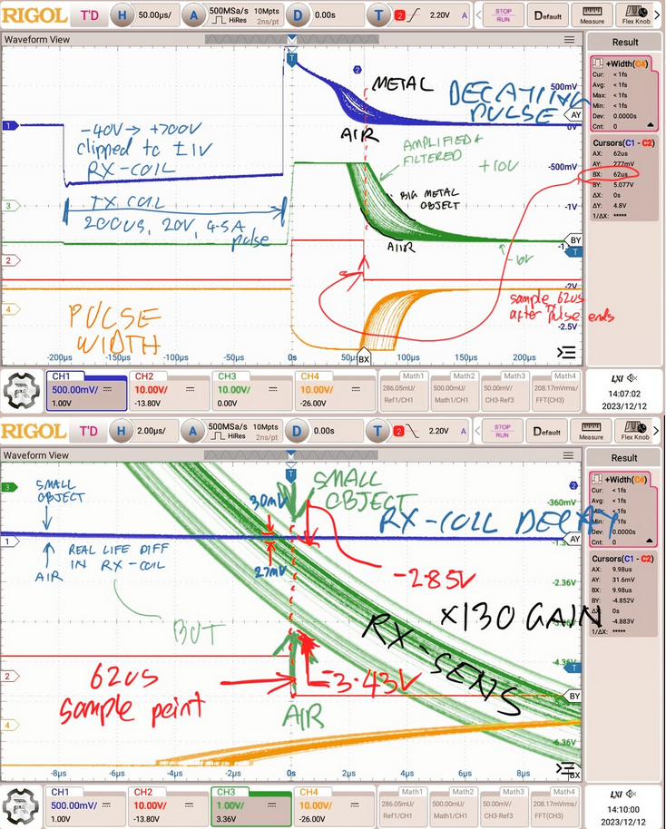
Following on from my previous post, here are the results.
The top chart, at 50 µs/div, shows a very large piece of metal—not a realistic test scenario but still impressive, packing a punch even at 0.5 m. The blue plot shows the received pulse decaying and highlights a sweet spot to measure changes: right at 62 µs after the TX pulse ends.
The second chart zooms in to 2 µs/div. At this level, only the value at 62 µs is relevant. At this point, the RX coil voltage (blue line) for air versus a small metal object is 27 mV and 30 mV, respectively. However, in the midst of the fuzzy noise, it’s nearly imperceptible—just a faint, straight-line difference.
Adding a few op amps to filter and amplify the signal, with a gain of x130, transforms the result into the green line. Now, the readings at 62 µs are 2.85 V for air and 3.43 V for a small metal object—a significant improvement.
4/1/24 Not Happy
Three prototypes later, and I’m still not entirely satisfied with the design. I can now detect a very small metal object at about 40 cm, but the system’s high gain makes it quite unstable. The RP2040, paired with a bit of Python, helps compensate somewhat, but it’s clear I’ll need something better if I want to fully automate the search process using Roverling Mk.ⅠⅠ.
Version 3 introduced targeted gain at a specific sample time after the impulse. Right now, the sweet spot seems to be at 47.6 µs, where I’m seeing a voltage change from about 220 mV to 225 mV. The Python code automatically adjusts the baseline, allowing me to amplify just the critical part of the signal. I even display the amplified result on an old-style meter driven by the RP2040 using differential PWM. However, the op-amps I’m using currently have a slew rate of around 13 V/µs, and I’d need something closer to 100 V/µs after amplification to properly resolve the ‘sweet spot.’
Now, Version 4 is on the drawing board. I plan to use higher-performance op-amps (since I now understand them much better) for the input and preamp stages. I’ve also decided to abandon the RP2040’s underwhelming 12-bit ADC. For $30, I can get a 24-bit oversampling ADC with a flat passband digital filter and external sync (critical for my application), with an SPI interface, made by Analog Devices. Honestly, I probably should have taken this route from the start.
11/1/2024 Fly-back Decay Curve
Version 5 is now underway, focusing on a full-scale read of the bottom 5 V of the fly-back decay curve. The coils have been redesigned, thanks to some fantastic online reference materials. Previously, RX coil response sampling couldn’t occur before 45 µs and was more reliable around 65 µs. With this new design—overlaying a circular receive coil under an elliptical transmit coil—mutual coupling has been significantly reduced, allowing sampling to begin at 10 µs. This is a major improvement, particularly for gold detection.
A big thanks to element14 for supplying the precision components. In theory, 32 bits of filtered data over 5 V should provide an LSB resolution in the range of 1.2 nV.
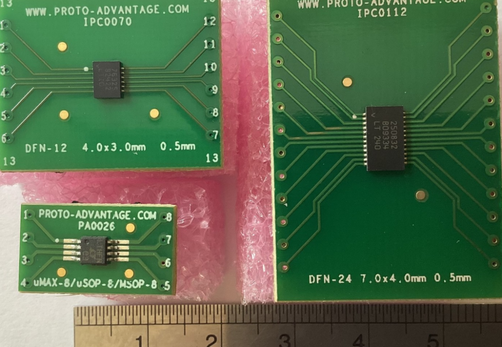
Next problem: these parts no longer come in DIL packages. They’re really small, and I’ll need to solder them by hand… wish me luck!
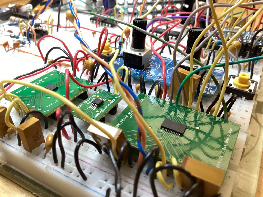
29/1/2024 Too Small
After numerous attempts to solder 0.2 mm wire onto 0.25 mm pads spaced just 0.5 mm apart, I’ve come to the conclusion that I need SMT-to-DIP adaptors. Luckily, I discovered Proto Advantage. Not only do they have all the adaptors I need for this project, but they’ll also procure and solder those tiny components onto the PCB for me.
Awesome! Now I’m just waiting on delivery from Canada.
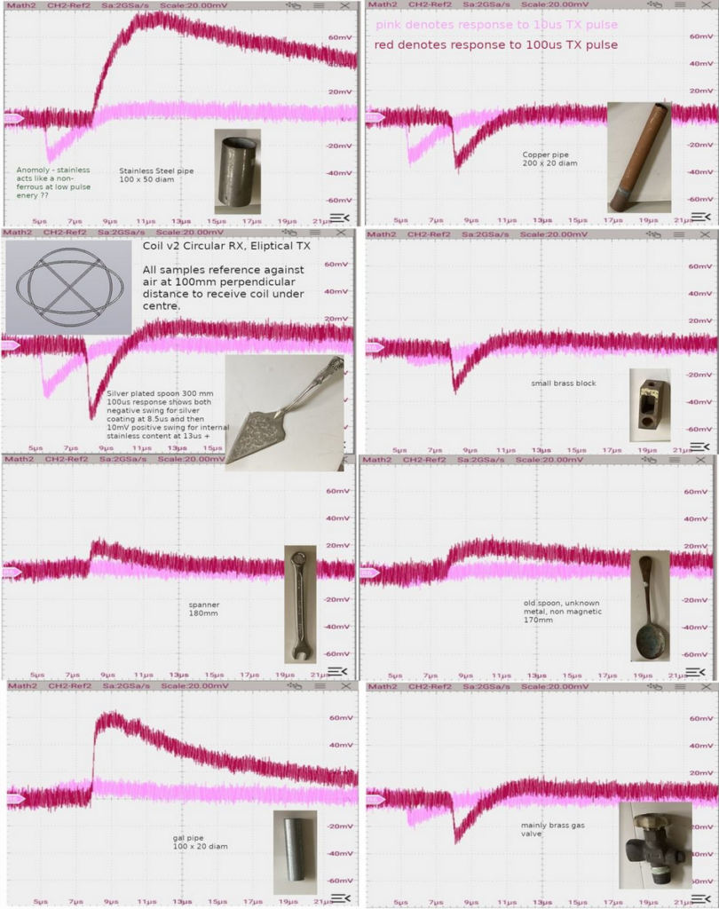
30/1/2024 New Coils
Version 2 coils have now been redesigned and are working extremely fast. Even with 2 m of RG62A/U coaxial cable, I can sample down to 7 µs. Discrimination is surprisingly effective, although I can’t test with gold yet since I don’t have any on hand. 🙂 The elliptical coil has proven to be a real game-changer for me.
From my research, most pulse induction detectors only examine the bottom 700 mV of the decay curve. However, in my testing and with my coil, I found the most useful information lies between 500 mV and 5 V. Not only is there significantly more information in this range, but it’s also well above the noise margin, making filtering far easier.
I also examined the response at voltages above 5 V. While I could sample 650 ns sooner in the best-case scenario, this only yielded a 10% improvement—hardly worth the additional effort.
31/1/2024 Finding the Sweet Spot
I conducted a controlled test to evaluate the discrimination characteristics of the dual elliptical coil design across various induction pulse periods. The charts display the difference between the baseline and the target object within the 5–20 µs sample period. The vertical resolution is set to 10 mV/div, with a noise component of ±10 mV.
Kicking goals now…
Test objects
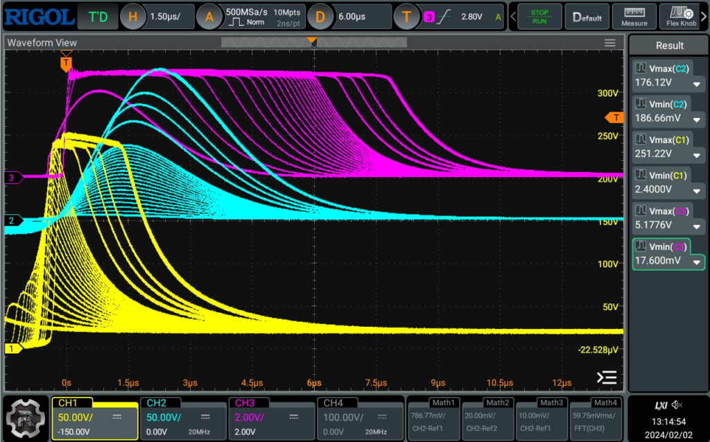
2/2/2024 High Voltage
Impulse response versus TX pulse width (h/w/v513) tested with the following increments: first 1–20 µs, then 30, 40, 50, and finally 100 µs.
Yellow: TX pulse, fly-back reaches 251 V
Blue: RX pulse, fly-back reaches 176 V
Pink: Conditioned sample, 5 V max
7/2/2024 Super Fast Sample Time
Automatic sample timing search: h/w v5.14 (RP2040 ADC), s/w v2.08, coil v2.01. The most optimal solution was determined using a natural logarithmic function. With a 5 µs pulse, sampling can begin at 4.5 µs, and with a 50 µs pulse, sampling starts at 7.6 µs, enabling the detection of non-ferrous metals.
The function used:
math.e ** (SampleIndex * 0.3) - 1
13/2/2024 Integration
The Pulse Induction Metal Detector (PIMD) project now meets Roverling MkII. Welcome to Stage 2: Integration.
After many months of development, I’ve managed to build a pulse induction metal detector from scratch. While I’m still waiting on better ADCs to arrive before designing a PCB, the PIMD works surprisingly well with the RP2040’s 12-bit ADC. With a transmit pulse ranging from 5–50 µs, I can sample as early as 4.5–7.6 µs, allowing for excellent discrimination between different metals. Taking it a step further, I can also roughly estimate the proportion of ferrous to non-ferrous material.
I’m using a 8×8-LED matrix as an indicator. This effectively serves as a colour-coded bar chart:
X-axis: Sample time (I take 20 samples, average them, and then apply an LPF at 8 distinct points).
The first point is determined by searching for the first time the RX return level drops to 95% of the initial detectable voltage.
The remaining 7 points are spaced using a natural logarithmic function that accurately matches the decay response.
Y-axis: The difference (in mV) between the current averaged sample and the reference sample.
Precise timing is critical, and I’ve managed to reduce sample timing jitter to under 10 ns. Python on the RP2040 isn’t ideal, as running the PWM frequency at 1 kHz introduces a rounding error (likely), causing 100 ns of jitter. However, switching to 2 kHz resolves this issue. For synchronisation between TX and RX, it’s also essential to use PWM channels from the same slice.
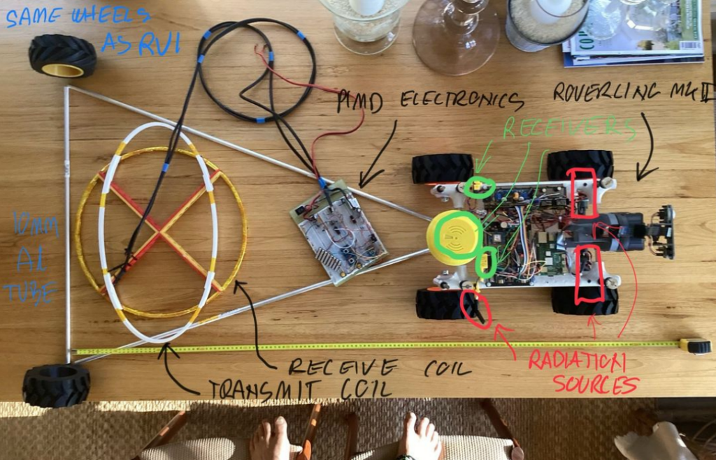
The next step is to integrate the PIMD with Roverling MkII. I plan to use a standard trailer configuration with a tow bar, suspending the sensor coil just above ground level. While I’d prefer carbon fibre or plastic for the frame, I’ll be using 10 mm aluminium rod for now (ensuring there are no loops). Although the PIMD can calibrate around this and maintain a reliable baseline, aluminium in the frame theoretically reduces sensitivity.
Roverling’s onboard electronics present some challenges:
Noise sources:
A radio transmitter.
Two unshielded 11W motors, generating significant interference.
GPS shielding: The GPS receiver on board is particularly sensitive to pulse noise.
To mitigate this, I plan to position the coils at least 0.5 m from the vehicle. The PIMD electronics, which are also highly sensitive, will be mounted halfway along the trailer for optimal isolation. Additionally, the 40 V vehicle power supply is too noisy, so I’ll be adding yet another Ryobi battery dedicated solely to the PIMD.
Time to fire up FreeCAD and start designing and printing more parts. Let’s get this prototype rolling!
15/2/1024 Massive Power Boost – 6yo Test Driver
Roverling MkII has had its power supply upgraded from 20 V to 40 V to provide the extra torque needed to tow the PIMD sensor trailer up hills. However, with this additional power comes increased speed—so naturally, I handed the controls over to a 6-year-old to test its stability.
Needless to say, I’ll be adding roll bars before any further “junior testing.”
19/2/24 Proto Advantage
Thanks, Proto Advantage—my parts have finally arrived from the US after three weeks in the post. Looks like my designs are no longer limited to through-hole technology components. Long live SMT!
Not only do they have all the adaptors I need for this project (and likely future ones), but they’ll also procure parts from DigiKey and solder those tiny components onto the PCBs for me.
24/2/1024 Oversample
The new oversampling ADC is now connected and provides two outputs: a 14-bit no-latency value and a 32-bit filtered and decimated value.
The next step was to determine whether the filtered output offers any advantage. The filtering process involves oversampling and decimation by a factor of 256, meaning at 2 kHz sampling, each sample takes roughly 125 ms. Additionally, seven sample periods are required to account for the group delay response to an impulse. This is compared to using eight different sample points at 120 samples per point—significantly more than I had initially planned.
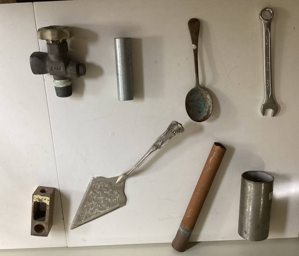
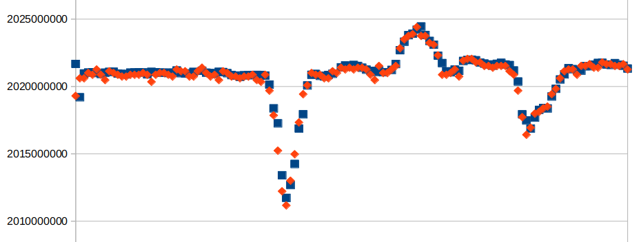
Both methods show a similar response to slow-moving metal objects:
The first dip is a silver spoon.
The next bump up is galvanised pipe.
The final dip is copper pipe.
The vertical scale for this comparison is 11.6 mV/div.
With all other variables held constant:
Noise in filtered samples (blue) is approximately ±450 µV.
Noise in raw samples (red) is approximately ±1400 µV.
The left scale represents the adjusted value for 32 bits, where V = x / 2^31 * 5, resulting in 465 µV/div.
The key decision is whether to pursue multiple sample times or a single sample time with higher resolution. While multiple sample times allow for better discrimination when ferrous and non-ferrous metals are present together, the only significant advantage occurs after the first sample time. Given this, it likely makes more sense to proceed with the single-sample approach for simplicity and efficiency.
26/2/2024 Making Progress
I’ve now coded the system to use the filtered 32-bit data after the initial baselining and sample timing is determined using the raw 14-bit data. The next step was to analyse the characteristics of different pulse widths as an object is passed over a period of 5 seconds. The horizontal axis of the chart represents time, covering about 30 seconds, while the vertical axis shows the integer representation of the ADC filtered value.
The results so far have been absolutely great! 🙂
Silver spoon and copper pipe: Both show identical responses for 20 µs and 40 µs pulses.
Ferrous pipe:
Almost no response at 10 µs.
Displays a strange “after-response” when the object is removed.
Increasing the pulse width results in an almost linear increase in sensitivity to ferrous objects but shows only a modest improvement in response to non-ferrous objects.
I’ve traded the ability to collect samples at 8 different points for higher resolution and less noise, but it seems there may be potential for greater discrimination by varying the pulse width. However, there’s one significant challenge:
Heat generation: At higher pulse widths, the system generates more heat. This heat causes slight drifting in the pulse-driving circuitry, which, in turn, leads to substantial drift in the sensitive receive circuitry.
Finding ways to manage the heat and mitigate its effects on circuit stability will be critical moving forward, especially if pulse-width adjustments are to be used for discrimination improvements.
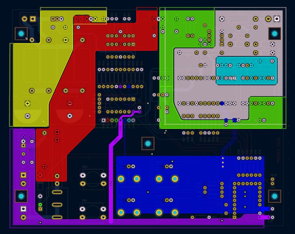
29/2/2024 Printed Circuit Board
It’s time for a PCB before any more fine-tuning to squeeze out those last few percent gains. I suspect the solderless prototype board is now the main contributor to the noise floor.
It’s been 20 years since I last designed a PCB, so there’s a bit of relearning ahead. Back then, I used the very expensive Mentor Graphics software on Apollo Unix Workstations. Now, I’m switching to KiCad—a free, well-supported tool with a large library, running on my free Ubuntu OS on an Intel platform.
While KiCad doesn’t have an auto-router, I’m not too concerned. I’ve always enjoyed the maze-like challenge of manually routing a tight board. I’m sure there will be plenty of frustrations along the way, but I’m looking forward to diving back into the process.
3/3/2024 Ryobi Battery Problem
Before designing the PCB, I needed to tidy up a few things. First, I shortened the leads to the coils from nearly 2 m (used for testing) to about 50 cm. As expected, this reduced the parasitic capacitance significantly, which was evident because the damping resistor on the transmit coil needed to be increased from 220 Ω to 490 Ω. This, in turn, made the coil even faster—now, with a 20 µs pulse, I can sample as soon as 5.8 µs, making gold detection easier.
Next, I replaced my bench power supply with a Ryobi battery pack, which I use for most of my projects. You’d think a modern battery would be quieter than my ancient power supply, but after a frustrating day of investigation, I discovered that’s not the case.
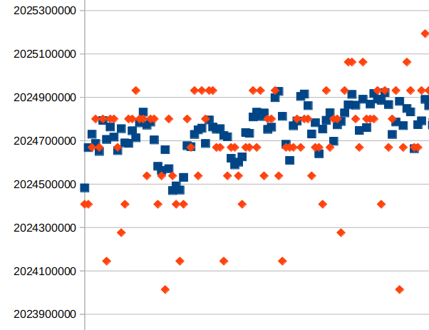
Every 128 ms, I collect a digitally filtered 32-bit representation of the decaying voltage. Most of the time, the measurements are very stable, with deviations of less than 1 mV. However, every 15 seconds or so, there’s a massive variation lasting about half a second, enough to ruin any accurate detection during that time.
In the measurements above, you can see the stability in the data, followed by a sudden, massive variation.
I connected the oscilloscope to the Ryobi battery pack, and even with no load, the battery exhibits a strange behaviour every 15 seconds. It appears to be performing some kind of internal check.
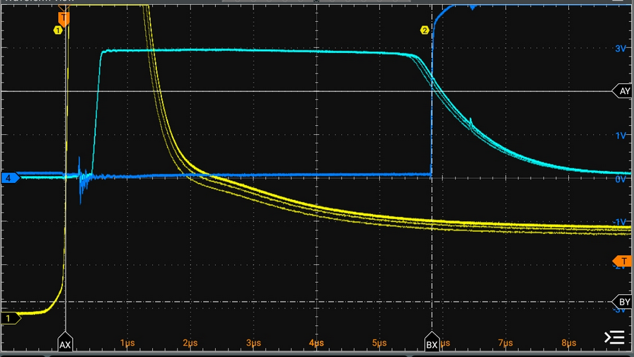
The yellow line marks the end of the excitation pulse, the green line represents the last 5 V of the received decay, and the rising blue edge shows the exact sample point. With persistence turned up, you can clearly see shadows in the transmit and receive pulses dipping briefly—enough to interfere with accurate detection.
Zooming in on the spikes reveals that each event lasts around 1 ms, with a voltage drop of nearly half the battery’s total voltage.
The Ryobi battery pack is clearly unsuitable for sensitive applications like this. I’ll need to find a quieter, more stable power source for this project. No more Ryobi battery packs for precision work!
9/3/2024 Drift
Next problem to solve – drifting component parameters, especially when going to full power on the drive circuitry. This phenomenon doesn’t work well with the static baselining I have been doing up to now, but it has it’s place for pinpointing edges so I’ll keep it in the system.
What I really thought I needed was a high pass filter. I found a much better solution using statistics, in particular the standard deviation function. In the below chart, the blue line is the filtered/decimated ADC 32 bit data, decimal scale on the right axis. The green is the standard deviation, and the red is the standard deviation multiplied by the sign of the difference of the sample at the beginning and end of the sample. Bottom scale is time in ms.
From left to right, first blue run with 20us pulse, passing samples at 150mm Ag, Fe, Fe, Ag. Next run turned up pulse width to 50us which heats up the power resistors somewhat. I didn’t wait for it to stabilise so drift down is evident. Samples Ag, Ag, Fe, Fe. You’ll notice a much bigger response to ferrous metals. Last run turned the pulse (effective power) down to 5us. Samples Ag and Ag followed by a hold over samples Ag & Ag.
The next issue to address isdrifting component parameters, especially when running the drive circuitry at full power. This phenomenon doesn’t work well with the static baselining I’ve been using so far. However, static baselining still has its place for pinpointing edges, so I’ll keep it in the system.
Initially, I thought I needed a high-pass filter to handle this issue. Instead, I found a much better solution using statistics, specifically the standard deviation function.
In the chart below:
Blue line: Filtered and decimated 32-bit ADC data (right decimal scale).
Green line: Standard deviation of the data.
Red line: Standard deviation multiplied by the sign of the difference between the sample values at the start and end of the sample window.
Bottom scale: Time in milliseconds.
First Run:
Pulse width: 20 µs.
Passed samples: Ag (silver), Fe (iron), Fe, Ag.
Stable operation, minimal drift.
Second Run:
Pulse width: 50 µs (increased power).
The power resistors heated up, causing noticeable drift (downward trend in the blue line).
Passed samples: Ag, Ag, Fe, Fe.
The response to ferrous metals (Fe) is much larger with the increased pulse width.
Third Run:
Pulse width: 5 µs (reduced power).
Passed samples: Ag, Ag, and then, Ag, Ag but slowly.
Using standard deviation and its signed adjustment provides a dynamic way to account for drift, without relying solely on static baselining.
Increasing the pulse width significantly improves ferrous metal detection, but it also introduces drift due to component heating. Conversely, shorter pulses reduce power consumption and drift but provide smaller signals.
14/3/2024 Power System Noise
Following on from the Standard Deviation edge detector, I’ve implemented a simple state machine to better detect changes and their direction. Now that this has been refined, it works very well up to about 20 cm, after which the noise becomes significant. It’s time to work on reducing noise, even though I’m still using a solderless breadboard.
The plan was to untether the USB connection used for code development, but that turned out to be harder than expected. Initially, I used the RP2040’s onboard flash memory to store data while disconnected, but this caused at least a 10-fold increase in the noise floor, even with an additional half dozen capacitors added. Once I identified the issue, I configured a single UART TX pin to output the data instead, eliminating the need for USB connectivity or onboard flash storage.
What surprised me most is that noise is about 50% lower when the RP2040 is powered via USB—either from a PC or a plug pack—compared to using the onboard 7805 regulator with the 20 V supply. Nothing I’ve tried has resolved this, and I suspect a proper PCB may help reduce the noise further.
Another major improvement came from changing the pulse and sampling frequency. I was initially using 4 kHz, but since it isn’t a prime number, there seemed to be a beat frequency in the noise. Changing to 3719 Hz reduced the noise by half.
Current baseline noise standard deviation over 10 samples in free air:
200 uV USB powered, no flash
250 uV Battery powered, no flash
900 uV USB powered, using flash
4000 uV Battery powered, using flash
16/3/2024 Critical Component
I accidentally blew up a critical component due to my dodgy solderless breadboard and loose wires. While I wait at least three weeks for the SMT replacements to arrive from Canada, I’ve decided to bite the bullet, relearn PCB design using KiCad, and finally get a proper PCB designed and manufactured.
30/5/2024 Creating Roverling Vehicle Control System
While waiting for replacement components, I began work on RV3, an updated version of Roverling based on the previous MkII, but specifically designed to operate autonomously with the metal detector.
It’s almost complete, but outdoor development has stalled due to rain. One of the final tasks is achieving accurate GPS steering. At the moment, I can achieve about 0.5 m accuracy, but for this project, I’ll need a GNSS RTK-capable module. I’m currently searching for a good but affordable option.
Fortunately, there are a couple of nearby government Continuously Operating Reference Stations, and their free NTRIP correction streams should allow me to achieve 2–3 cm accuracy.
8/7/2024 Roverling in Control
It’s taken some time, but the Roverling control system is now working well.
The first level of control uses a magnetometer, calibrated offline using all three axes for sphere re-mapping, and then calibrated again on the Roverling itself using only the X and Y axes with a figure-of-eight manoeuvre. However, the magnetometer is only accurate when horizontal, which is problematic when Roverling is navigating up, down, or across hills. To address this, tilt compensation is applied based on pitch and roll, which are derived from a three-axis accelerometer. Unfortunately, the accelerometer can only determine pitch and roll while stationary, which isn’t helpful when moving.
The next level of control comes from the GPS. While helpful, there are still limitations until I can integrate an RTK module. For now:
The best update interval is once per second.
Precision is around 18 cm.
Accuracy, after locking onto approximately 20 satellites and allowing 15 minutes to stabilise the fix, is about 50 cm.
While there’s room for improvement, the system is good enough for now.
The chart below shows GPS position during fully autonomous control:
First test: A 40 m run on a varying 10-degree slope. Roverling stays within a 1 m corridor.
Second test: A series of ‘slots’ on flatter ground, 10 m long, with tight turning circles at each end. Again, Roverling maintains a 1 m corridor.
It’s a promising start!
12/7/2024 PCB Arrives
The first PCB I’ve designed in many years has arrived and is working with only a few minor issues. I’m now in the process of testing and calibrating it.
So far, it looks like I’ve managed to achieve a minimum sampling delay of around 4 µs and approximately 10 µV of precision on my timed 32-bit ADC sampling.
A great step forward!
1/8/2024 First Integration Test
The first integration test is complete! The power systems are working well, and RS232 communications between the PI trailer and Roverling are solid. I’m getting 30 updates per second from the PI’s 32-bit ADC via LoRa, streaming back to my desktop computer.
However, there’s an issue: it seems the coils are too loose, and the wires are shifting relative to each other during the shaking and bumping. To address this, I’ll coat the wiring in epoxy to stabilise it and also work on making the trailer lighter.
A few more tweaks, and it should be ready for further testing!
23/12/2024 New Coil Design – Version 3
I’ve gone back to basics with a version 3 coil, focusing on making it stable. This design consists of two rectangular coils epoxied onto a 6.25 mm glass substrate, protected underneath by a polycarbonate sheet.
Transmit Coil:
Dimensions: 520 x 360 mm
10 turns of 0.5 mm (24 AWG) enamelled magnet wire
Length: 17.6 m
Resistance: 1.7 Ω
Receive Coil:
Dimensions: 430 x 265 mm
50 turns of 0.25 mm (30 AWG) Teflon-insulated, silver-plated copper wire-wrap wire
Length: 30.8 m
Resistance: 22.9 Ω
Many designs I’ve seen include a series resistor in the drive circuit for the TX coil. I experimented with this and found that reducing the resistor from 9.4 Ω to zero only slowed the response by 0.6 µs but significantly increased depth penetration.
Although this version performs well on the bench, it’s very heavy, and the front-wheel-drive Roverling struggles to maintain traction. I’ll need to revisit the design to reduce the weight while maintaining stability.
2/1/2025 New Coil Design – Version 4
I’m exploring alternative materials and techniques to develop a better solution for keeping the coils rigid while reducing weight.
The Version 3 coil, while stable and functional, proved to be too heavy for the front-wheel-drive Roverling, causing traction issues.
The goal is to maintain stability and durability without compromising the performance gains achieved in the previous version. Time to get prototyping!
16/2/2025 Field Tests
Coils v4 is now complete. I used a piece of 12mm thick perspex and had slots routed to house the coils. The receive coil is shielded by copper tape, and then both coils are embedded in perspex. For the initial field testing I’ll use this ‘pusher’ and a laptop to monitor using this newly created GUI.
I have now developed a Python-based GUI to interface with the RP2040 acquisition MCU. The timing between the removal of the transmit pulse and the subsequent acquisition of the receive pulse is accurate to within 15 ns. Once the coils and circuitry have warmed up, the standard deviation of the received signal is typically better than 100 µV.
The slope seen in the data below is due to the system still warming up. Nonetheless, it’s clear that ferrous metals (steel spanner) are detected as positive spikes, while non-ferrous metals (piece of copper pipe) produce negative spikes. The polarity difference happens because ferrous metals store magnetic energy, reinforcing the decay field (positive spike), while non-ferrous metals induce opposing eddy currents, weakening the field (negative spike).
Through testing, I’ve found that the optimal setup is a 40 µs transmit pulse, generating a peak current of 7 A. Sampling at 8.4 µs provides the best results, as this is when the 100V+ signal has been critically damped to around 3V. The system runs at a 5 kHz pulse rate, with a decimation filter of 256, providing 20 samples per second.
I’ve already detected a few large underground spikes but haven’t dug them up yet to see what they are.
22/6/2026 — Back from the Shelf
It’s been over a year since my last entry. I kind of lost interest and got busy on other projects.
Where I left off it actually worked in the field. I found a 90-year-old brass dipstick about 30cm down, an old buried enamelled steel plate and some sash window weights, pushing the coil on wheels around and watching the laptop. No real ground discrimination, just doing it manually from the GUI.
Then a couple of things happened that completely changed the trajectory.
For a very short period I got access to Fable 5, Anthropic’s newest model. I wanted to give it a real test, so I looked through my project directory for something meaty and maybe unfinished. I found PIMD and thought that will do. I fed in the Python source code, all my notes, this diary, schematics, screenshots, oscilloscope plots, etc. I then asked Fable to do a deep review against commercially available equipment, specifically pointing out good and bad points. Was I even in the ballpark?
It pointed out some flaws, but also uncovered things I wanted to do but didn’t — mainly because of the programming effort required. I knew I would be fighting Python at this level, and it would take me forever. But the other thing I have wanted to do for a while was to learn how to use Claude Code.
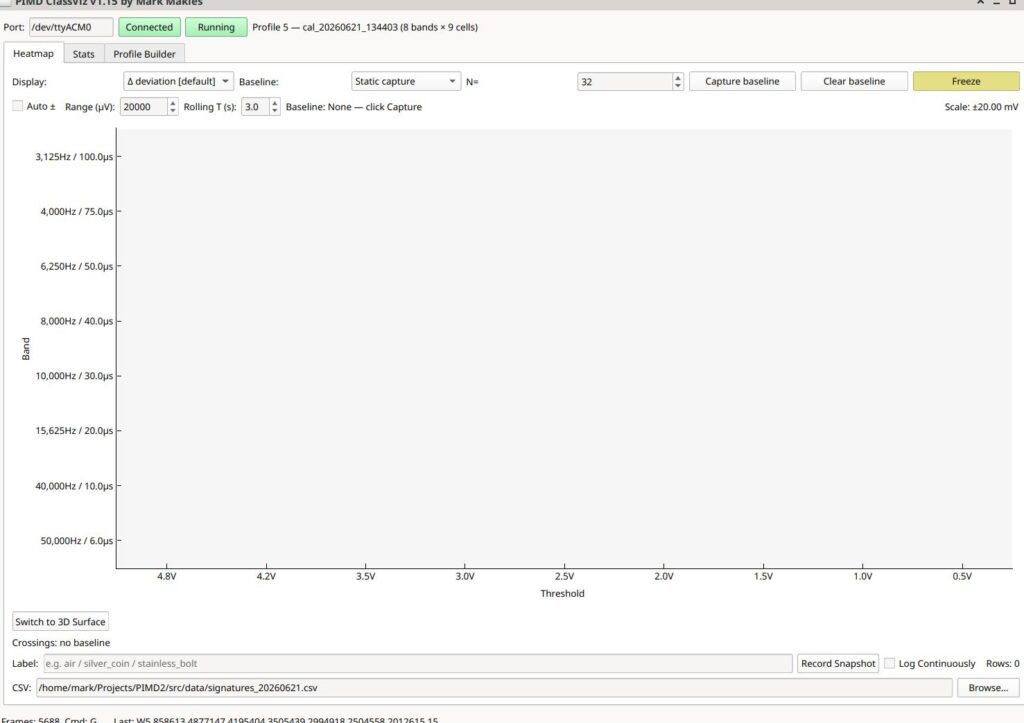
So inside a week all the bugs and mistakes with my firmware and GUI were sorted out, and new functionality added, which I could never have done myself in a reasonable time. Two new PC apps were created: pimd_delaycal.py, which automatically determines exact timings for acquisitions, and pimd_classviz.py, a tool to visualise the data. The aim is to eventually get these vectors into ML for classification and ground discrimination.
I got AI to do another review and now it’s calling it
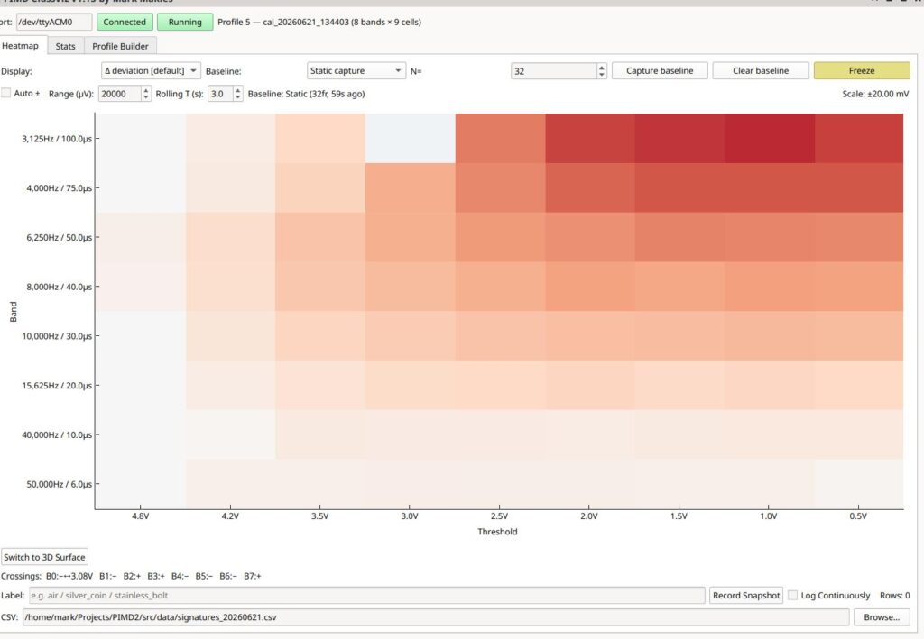
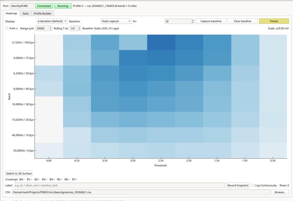
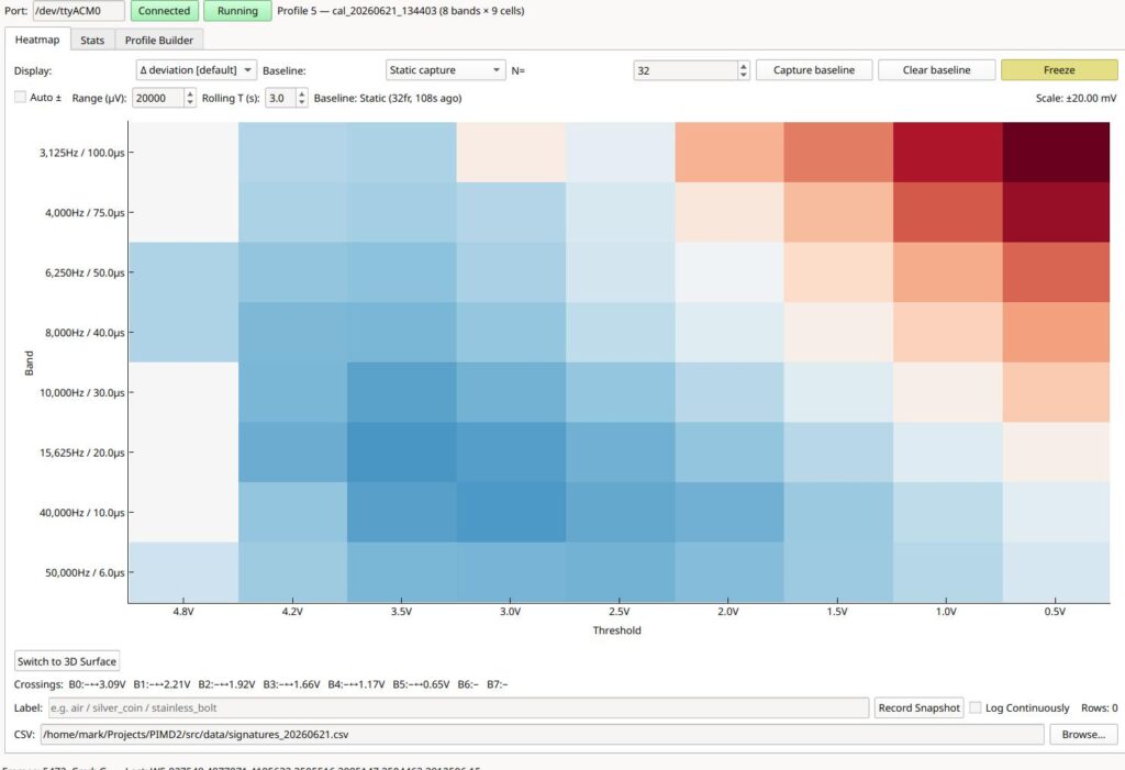
ClassViz Output top row: Air, Spanner, Copper Pipe. Bottom, both copper and steel targets.
I’ve decided to publish everything to date on GitHub: the firmware, the three PC tools, the KiCad project, a full engineering reference and the per-tool docs. It’s a work in progress, but someone may find it useful.
Next step, me learning machine learning. The entire point of that n-cell matrix is that it’s built from the ground up to be a classifier input, for filtering, for ferrous/non-ferrous classification and for the real stretch goal, ground discrimination.
There’s some refinement to come, possibly trimming the cell count for a faster response, but only once I’m certain I’m not throwing away hidden information in those extra cells, and a front-end revision to retire a 1990s MOSFET I’ve been running rather harder than its datasheet would like. And one day design a proper PCB.
So much has changed in the update – best to consult Change Log in GitHub to get up to speed.
PC Gamer: “I have seen the future, and it’s this 3D-printed air raid siren honking its baleful tones over my neighbourhood as the waters rise”
Why Build a Siren?
I made a VERY loud portable motor-driven siren because:
I had some spare RC parts, I’m a big fan of repurposing functional bits rather than throwing them out.
I just got my first new 3D printer, a Prusa
I wanted to make something cool.
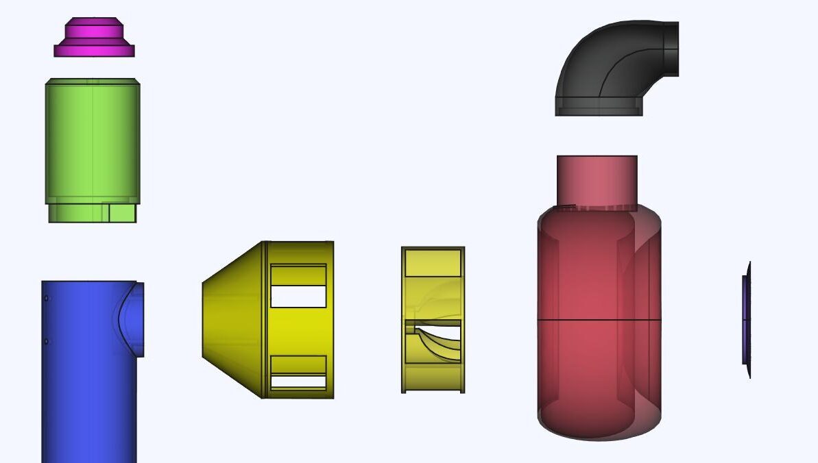
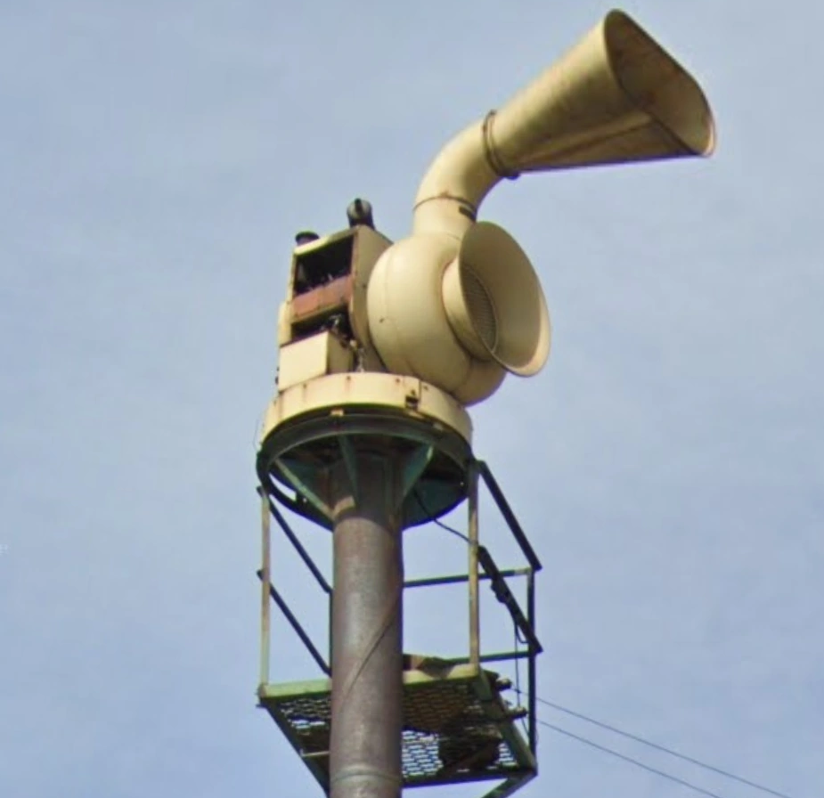
And finally I saw a picture of an air raid siren, I thought, “I can make that “
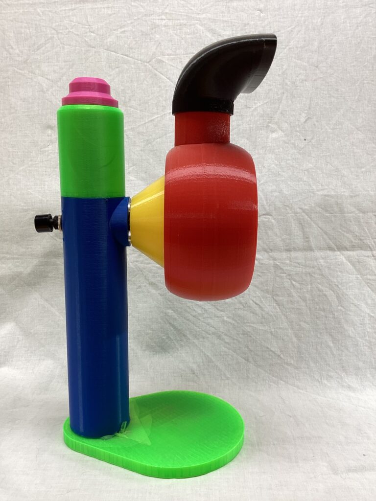
The result? A ridiculously loud and fun build with surprising practical applications. While this is far from a “refined” design, it’s proof of concept—and with a little know-how in electronics, some soldering skills, access to a basic 3D printer, and a few RC components, you can make one too.
The overall shape of my design was influenced by a picture of a massive Cold War-era siren, which I later discovered to be an ACA (Alerting Communications of America) Allertor 125. Its bold, retro aesthetic and functional design inspired me to create this scaled-down, portable version for the project.